Generating Random Numbers from Custom Probability Distributions
STELLA® and iThink® provide many useful probability distribution functions (listed here). However, sometimes you need to draw random numbers from a different probability distribution, perhaps one you have developed yourself. In these cases, it is possible to invert the cumulative probability distribution and use a uniformly distributed random number between zero and one (using the RANDOM built-in) to draw a number from the intended distribution. With a lot of math, this can be done analytically (briefly described here). With no math at all, it can be closely approximated using the graphical function.
Find the Cumulative Distribution Function
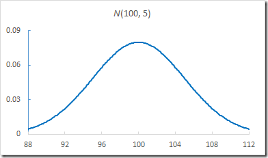
Every probability distribution has a probability density function (PDF) that relates a value with its probability of occurring. The most famous continuous PDF is the bell curve for the normal distribution:
From the PDF, we can see that the probability of randomly drawing 100 is just under 0.09 while the probability of randomly drawing 88 or 112 is close to zero. Note that applying the techniques described in this article to a continuous probability distribution will only approximate that distribution. The accuracy of the approximation will be determined by the number of data points included in the graphical function.
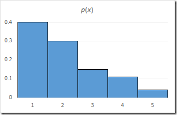
For discrete probability functions, the PDF resembles a histogram:
From this PDF, we can see that the probability of randomly drawing 1 is 0.4, while the probability of drawing 3 is 0.15. As discrete probability distributions can be represented exactly within graphical functions, the remainder of this article will focus on them.
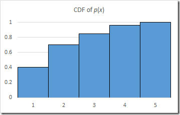
In contrast to the PDF, the cumulative distribution function (CDF) gives the probability of randomly drawing a number less than or equal to the given number. It is the integral of the PDF, i.e., at any point it is the area under the PDF curve up to that point. Necessarily, the y-axis always goes from 0 to 1. The CDF for the discrete probability distribution p(x) above is:
This shows that the probability of getting 3 or less is 0.85. That can be useful, but more important to our purpose, if we invert the CDF, we can draw random values from the distribution p(x).
Invert the Cumulative Probability Distribution
To analytically find the inverse of continuous function, we replace x with y and y with x in the equation and then solve for x. For discrete functions, however, we only have to swap the x and y columns of the table of values. The table of values for the above CDF is:
| x | CDF |
| 1 | 0.40 |
| 2 | 0.70 |
| 3 | 0.85 |
| 4 | 0.96 |
| 5 | 1.00 |
Therefore, the table for the inverse of the CDF is:
| CDF | x |
| 0.40 | 1 |
| 0.70 | 2 |
| 0.85 | 3 |
| 0.96 | 4 |
| 1.00 | 5 |
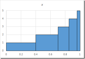
Graphing this, we get a better idea of what we just did:
This converts a uniformly distributed number between 0 and 1 into the desired discrete probability distribution p(x).
Using it in STELLA or iThink
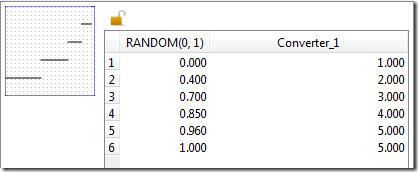
To use this in the software, create a graphical function with the equation RANDOM(0, 1), select the discrete graphical function type, unlock the x-values in the Points tab, and paste or enter the values in the Points tab. For this example, we need six points because discrete graphical functions require one extra point at the end that indicates where the final value ends:
Note the lock was unlocked by clicking on it once. If you don’t do this, you will not be able to change the x values. The x values, when entered, must be strictly increasing, so it would not be possible to type in 0.9 for the x value of point 3. To select a discrete graphical function, choose the third graphical function type at the bottom of the panel:
As stated earlier, this can also be used for continuous probability distributions if you are willing to sacrifice some accuracy. For these cases, you would choose the first graphical function type, which is the continuous graphical function (without extrapolation).
Verifying the Distribution is Correct
To test the distribution is working, connect the created graphical function (I named it value) to another converter. Array the second converter with a dimension X that encompasses the entire domain of p(x). In this case, the size of X must be 5 so there is one array element for each of the possible drawn values 1, 2, 3, 4, and 5. Set the equation of this converter to:
IF (Converter_1 = X) THEN PREVIOUS(SELF, 0) + 1 ELSE PREVIOUS(SELF, 0)
Change the Run Specs of the model to run from 1 to 10,000 with DT = 1. After the running the model, you can hover over the array to get the number of occurrences of each value across 10,000 draws (or you can put the array in a table). When I did this (using this model), I got:
| x | Occurrences | Frequency | p(x) |
| 1 | 4000 | 0.400 | 0.40 |
| 2 | 2966 | 0.297 | 0.30 |
| 3 | 1506 | 0.151 | 0.15 |
| 4 | 1124 | 0.112 | 0.11 |
| 5 | 404 | 0.040 | 0.04 |
As can be seen, the distribution as entered into STELLA/iThink correctly reproduces p(x).
