Skip to content

Making Connections

isee systems blog

Making Connections

  • About
  • More Connections
Search

COVID-19: Modeling Distributions of Incubation and Recovery Times

Updated: April 3, 2020April 1, 2020Filed under: Modeling Tips
  • STELLA & iThink
Comment

There is a flurry of models becoming available for the coronavirus pandemic we are in the midst of.  We at isee systems have issued our own, available here.  We’ve noticed a number of people use the canonical Susceptible-Exposed-Infected-Recovered (SEIR) model (in its simplest form):

seirWe’ve used this same model, albeit with disaggregation of severity of infection and the population that has been tested.  We observed with our model that the simple first-order material delay used to model Exposed people becoming Infected and Infected people becoming Recovered is not appropriate for this situation and has a significant impact on the results.  We chose to use an infinite-order delay, but that also is not quite right.

When choosing the order of a delay, one should consider the distribution of times around the specified delay time.  An infinite-order delay will delay all material for exactly that amount.  However, lower-order delays will delay material according to a distribution.  The shape of that distribution can be discerned with a PULSE.  As you can see in the graph below, the first-order material delay releases a large fraction of material almost immediately.
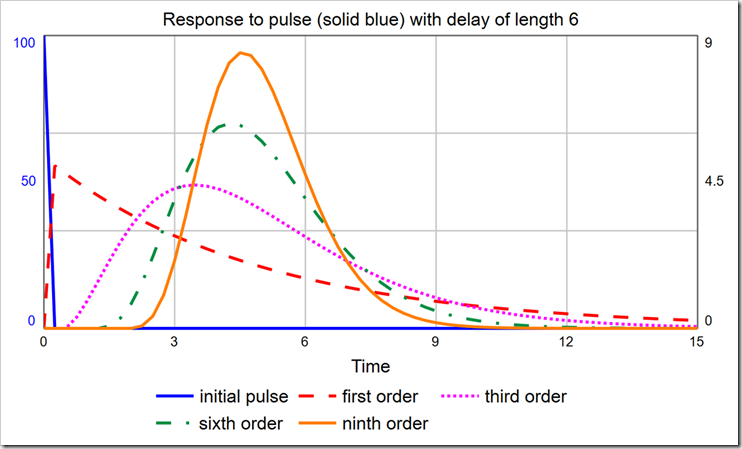
imageWith a delay time of six, the modes for the 1st-, 3rd-, 6th-, and 9th-order delays are, respectively:  DT (0.25), 3.5, 4.25, and 4.5.  It is certainly not true that the largest group of people who become Exposed move on to being Infected almost immediately (after one DT).  To correct this, we must use a higher-order material delay.  Notice the 3rd-, 6th-, and 9th-order delays are all skewed right (their peaks are not centered on the actual delay value, which is six, and they are asymmetric).  You can pick the order that most closely matches the actual distribution of, for example, time to show symptoms.  The latest data I saw said that the average time to show symptoms is 5 days, but many cases can be 14 or more days.  This indicates a long tail on the right side, making a 3rd- or a 6th-order more appropriate than a 9th-order.  It would be ideal, though, if we could experiment with different distributions just by changing the order.

Normally, we would explicitly expand the model to handle a higher-order delay.  However, consider that a 3rd-order delay requires three stocks, and a 6th-order requires six stocks, instead of just one.  This muddies up the diagram quite a bit and does not give us the flexibility to easily change the order because any change requires a change to the model structure.  The alternative is to use the DELAYN function, which allows you to specify the order of the delay as a parameter.  The problem with this approach is that you only have access to the output of the delay (a flow); you no longer have access to the contents of the stock.  In this application, we need to see how many people are Exposed and Infected.  In Business Dynamics, John Sterman proposes the following structure for this exact circumstance:
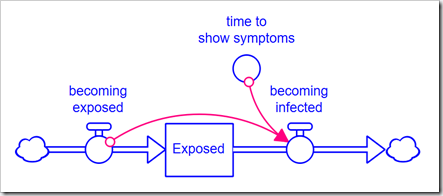
imageRather than formulate the outflow becoming infected as a draining process (based on the stock), it is formulated from the inflow using the equation, for example, for a 3rd-order delay:

DELAY3(becoming_exposed, time_to_show_symptoms, 0)
(more…)

Modeling Tips, STELLA & iThinkLeave a comment

Multiobjective Optimization

Updated: January 23, 2018January 9, 2018Filed under: Modeling Tips2 Comments

This is the third of a three-part series on calibration and optimization. The first part can be accessed here. The second part can be accessed here.

Sometimes optimizing one objective does not give the best solution, for example, when judgment is needed to determine which solution between many equally optimal solutions is truly the best, given the tradeoffs between them. While it is possible to approximate the tradeoffs by assigning different weights to each objective in a single-objective optimization, it is quite likely this will not find the best solution for your situation. In these cases, it is best to use multiobjective optimization, i.e., optimize for multiple objectives at the same time.

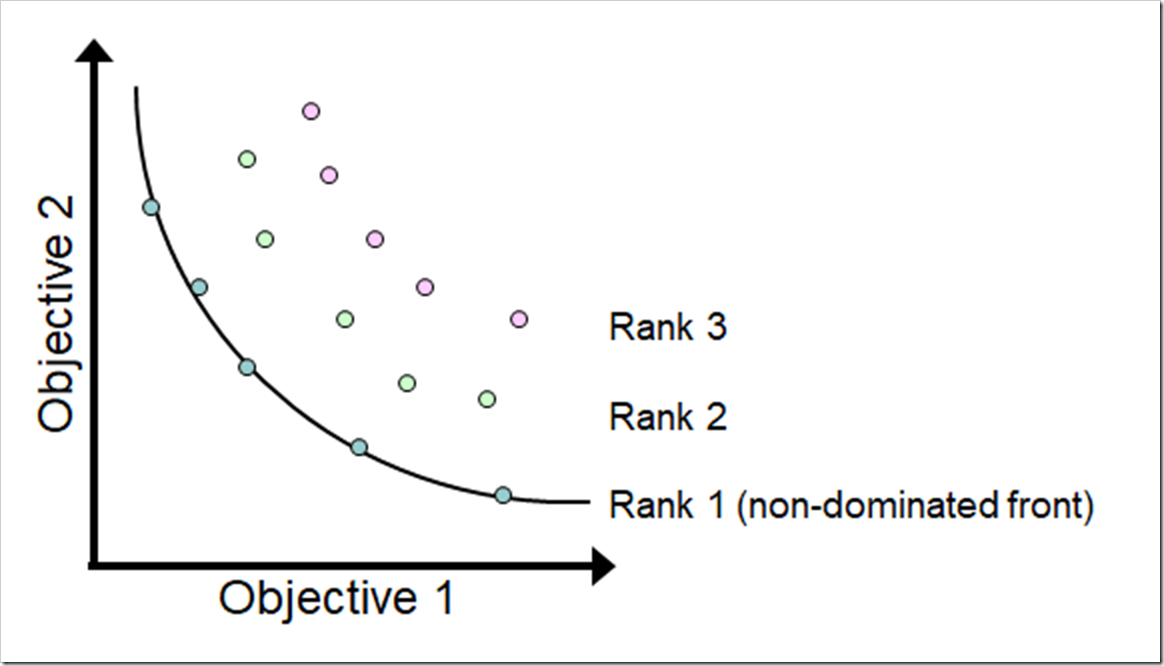
But what does that mean in practice? While I can find the optimal value of each objective, what does it mean to optimize all of them simultaneously? It certainly isn’t true that they will all be at their individual optimums when all are optimized. In fact, when we perform multiobjective optimization, we find a set of solutions that are all optimal according to the following definition of non-dominated:

A solution that outperforms another solution in at least one objective is non-dominated by the other solution.

The set of non-dominated solutions in the population are called the non-dominated front.  A non-dominated front (Pareto rank 1) for a minimization problem is shown in the figure below. Note there are also two dominated fronts in the set of solutions (Pareto ranks 2 and 3). The characteristic convex shape clearly shows the tradeoffs between the two objectives with the best compromise landing at the middle of the bend in the curve (called the knee). Beyond the knee in either direction, you experience diminishing returns.

image

The goal of a multiobjective optimization is to push all of these solutions toward the non-dominated Pareto front, which is the ideal set of optimum solutions. Be aware that you cannot be sure – without knowing the Pareto front – that the final set of non-dominated solutions from a multiobjective algorithm reached the Pareto front. However, you can test if running for additional generations improves the set of solutions (i.e., moves closer to the Pareto front).

While it is possible to optimize for many objectives simultaneously, it becomes somewhat impractical to optimize for more than three objectives:  a) as the number of objectives increase, the population size must increase exponentially and the number of generations must increase significantly (the computation time increases combinatorially as the number of objectives increase) and b) it is difficult to visualize the non-dominated fronts when you exceed three dimensions. The discussion in this post will be restricted to two objectives.

The Problem

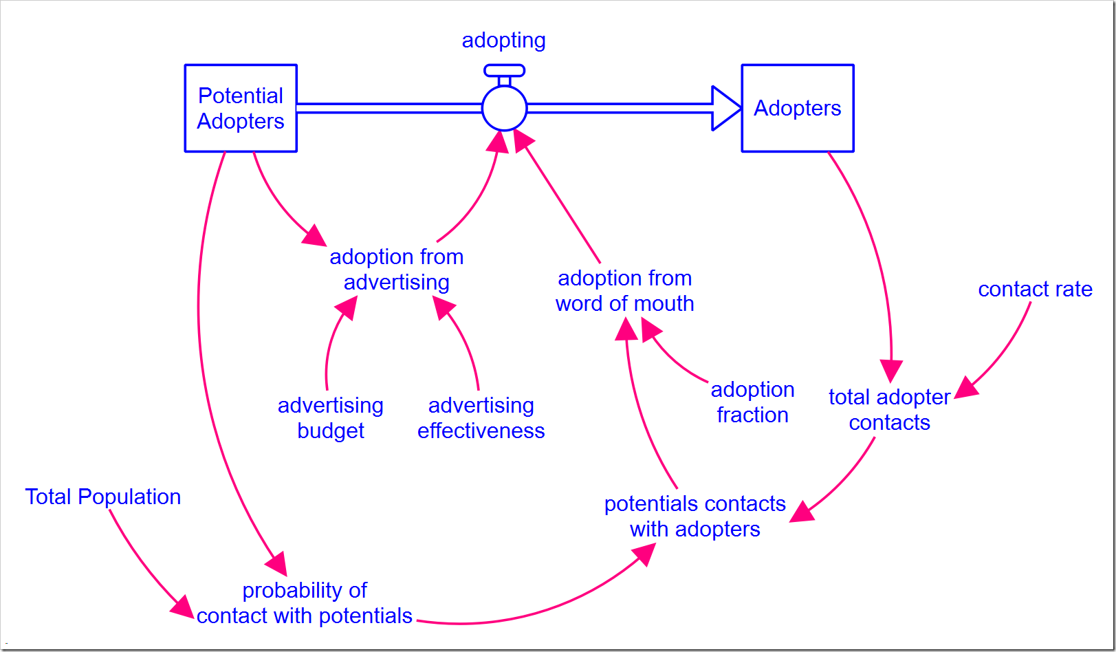
In the Limits to Growth series, we explored the Bass diffusion model. The model is shown again below and can be downloaded here (with all the changes described in this post).

image
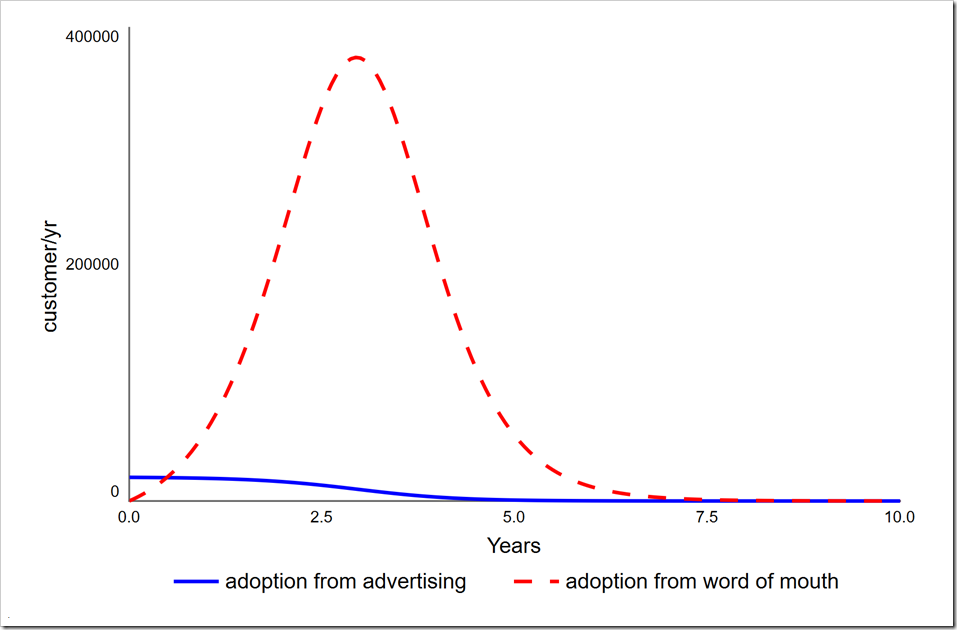
As you may recall, customers are converted by both advertising and word of mouth. In the closing post of that series, I discussed the importance of marketing spend to get the ball rolling. Specifically, without it, growth is very slow. Additionally, as more customers are converted, the word of mouth effect dominates how fast the product is adopted, making the marketing spend less and less effective. By effective, I specifically mean that it results in conversions. The graph below shows the two components of adopting and how the dominance shifts from marketing spend to word of mouth only six months after the product launch.

image

Note how the number of adoptions through advertising decreases over time. This suggest it is not necessary to continue advertising spend at the same level indefinitely. There is perhaps an optimal point where we could start to phase it out. [Warning: This scenario represents the adoption of a single durable good that is never replaced or updated. The situation is clearly different for both consumable goods and durable goods that are regularly replaced.]

If we are launching this unique product, say, the Pet Rock, we would be very interested to know whether we can increase our product lifetime profits by investing less in advertising. We can run an optimization that seeks to maximize conversions and minimize advertising spend over the life of the product.

(more…)

Modeling Tips
  • Bass diffusion
  • calibration
  • data
  • market dynamics
  • optimization
  • Stella
2 Comments

Optimizing Model Performance

Updated: January 9, 2018December 22, 2017Filed under: Modeling Tips2 Comments

This is the second of a three-part series on calibration and optimization. The first part can be accessed here. The third part can be accessed here.

Part one of this series explored calibrating a model using the Stella® Architect/Professional optimization feature (introduced in version 1.5). This post will explore using this same feature for single-objective optimization.

The Challenge

Last year, I explored the Shifting the Burden archetype with the example of using credit card debt to pay current expenses. In that case, adding feedback between expenses and an ability to pay allowed the credit card debt to stabilize. What if we instead wanted to maximize our savings and/or minimize our debt? The original model is shown below for reference and can be downloaded here (with the optimization configurations described below).

Most of these parameters cannot be adjusted by the person trying to control their debt. The interest rate and the minimum payment parameters are set by the credit card company. Let’s assume the income cannot easily be adjusted either, for example, by working overtime or taking on a second job (as we did before). That leaves only the spending rate, which we varied last time, and the minimum bank balance. The latter, you may argue, is set by the bank, but different banks and different bank accounts have different minimums…before they impose a charge. The balance can still fall below the level the bank sets.

We will perform two separate optimizations:  maximize savings (i.e., bank balance) and minimize credit card debt. We should not expect them to give the same results.

(more…)

Modeling Tips
  • calibration
  • data
  • optimization
  • Stella
2 Comments

Posts navigation

  • 1
  • 2
  • 3
  • 4
  • …
  • 29
  • Next

Categories

  • Education (4)
  • isee NetSim (3)
  • isee.NET Framework (1)
  • Modeling Tips (32)
  • News & Announcements (15)
  • STELLA & iThink (14)
  • Stories from the Field (5)
  • Systems Thinking (8)
  • Training (6)

Archives

Browse by keyword

2D array archetypes arrays Barry Richmond Bass diffusion builtins calibration Causal Loop CLD command line conferences crisis data diffusion Education environment export game graphical function h1n1 healthcare housing import iThink/STELLA market dynamics MODSIM modules mortgage netsim optimization Physics policy price releases scholarship software spatial Stella storytelling System Dynamics Society Systems Thinking Version 9.1.2 video webinar workshop

Recent Posts

  • COVID-19: Modeling Distributions of Incubation and Recovery Times April 1, 2020
  • Multiobjective Optimization January 9, 2018
  • Optimizing Model Performance December 22, 2017
  • Calibration in Stella® December 15, 2017
  • Drifting Goals March 9, 2016

RSS System Dynamics Forum

Recent Comments

  • best apps review on About
  • digital software on Modeling the Economic Crisis
  • Mishawaka Indiana on What are “Mental Models”?
  • La Paz Indiana on XMILE – An open standard for system dynamics models
  • Bristol Indiana on Modeling the Economic Crisis

Meta

  • Log in
  • Entries feed
  • Comments feed
  • WordPress.org
Products
Software (v1.3)
  • Stella Architect
  • Stella Professional
  • Stella Designer
  • Stella Simulator
  • iThink
  • Feature Updates
  • Policies
  • Publishing Options
  • License Agreement
Free Software
  • Stella Online
  • isee Player
  • Stella Architect Trial
Solutions
Consulting
  • Systems Innovation Practice
Common Applications
  • Business
  • Education
  • Research
  • Government
  • Energy
  • Health
  • Agriculture
  • Manufacturing
  • Conservation
Quick Links
About
  • isee systems
  • Systems Thinking
  • Barry Richmond Scholarship
Resources
  • Frequently Asked Questions
  • Product Help
  • Examples
  • Request Support
  • Request Quote
  • Systems in Focus
  • Quick Tips
  • Legacy Tutorials
News and Events
Upcoming Workshops
  • Introduction to Dynamic Modeling
  • Whole Systems Partnership
Newsletter
  • The Connector
Recent Webinars
  • Model Mysteries
Recent Training
  • Systems Thinking Practice
Press Release
  • Stella Architect Release

  Phone: (603) 448-4990   Email: info@iseesystems.com

   Monday - Friday: 9:00 am - 5:00 pm EDT | Saturday - Sunday: Closed
Wheelock Office Park | 31 Old Etna Rd, Suite 7N | Lebanon, NH 03766 | US

isee systems inc. holds registered trademark rights over the following: iThink®, STELLA®, Stella®, isee systems® and claims the following trademarks; isee NetSim™, Stella Live™, Causal Lens™ and Stella Online™.

Terms of Use

© 2017. isee systems inc . All rights reserved.