Tip: Setting up imports for 2D Graphical Functions
iThink and STELLA version 9.0 introduced a powerful new feature: data import and export with Excel. Here at isee, we were excited to hear from our customers about how much they appreciated the feature and how easy it was to use. In fact, many customers told us that it was the major reason they upgraded to version 9.0

Setting up a data import from Excel is pretty straight forward: type the name of the model variable in one cell, type the value you want to import in the cell below it, (or beside it if you are using horizontal orientation):
If you are importing a time series or graphical function, you just keep listing the data points in the cells below the variable name:

This kind of data formatting works well since an Excel sheet is made up of columns and rows. But how do you format data that is harder to visualize? Things get a little tricky when you start dealing with arrayed variables. The most complex import is a 2 dimensional array of graphical functions. It’s actually 3 dimensions!
I’ve put together a simple example to illustrate how to do this.
Let’s say you have a model set up to look at 3 teams’ performance on 3 different projects. The model has an array of Projects and Teams. The Project dimension has 3 elements: Project 1, Project 2 and Project 3. The Team dimension has 3 elements: Team 1,Team 2 and Team 3.
In this model we’ll put down a converter called “Performance rates” which we’ll later define as a 2D array of graphical functions over time. The converter will contain historical data on the various teams performance rates for the various projects.
You can see how this sort of setup is pretty close to what someone would want to do – track performance over time per project per team.
The format of the Excel spreasheet would look like this:
| Project 1 | Project 2 | Project 3 | ||||||
| Team 1 | Team 2 | Team 3 | Team 1 | Team 2 | Team 3 | Team 1 | Team 2 | Team 3 |
| Performance rates | … | … | *** | … | … | *** | … | … |
| 100 | 34 | 63 | 98 | 87 | 18 | 20 | 14 | 3 |
| 45 | 25 | 78 | 69 | 35 | 99 | 25 | 13 | 25 |
| 67 | 53 | 23 | 100 | 43 | 78 | 98 | 55 | 76 |
Notice that the Team 2 and Team 3 columns have an ellipsis (…) in the header that indicates the column is still part of the Project 1 array element. Start the next array element, Project 2 with 3 asterisks (***) at the top of the column.
This is important: The converter name is listed first, then then an ellipsis for each element of the team dimension, (since Team is our first dimension). The Project dimensions are delimited by the *** and of course the time data goes down.
After setting up your spreadsheet, you need to set the converter correctly.
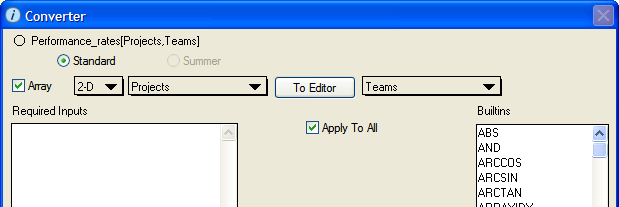
Converter Dialog:
In the converter dialog, first check Array, change it from 1D to 2D, (Teams and Projects) and leave Apply to All checked.
Click on the “Become Graphical Function” button on the lower left. This will switch to the Graphical Function dialog.
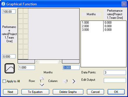
Graphical Function Dialog:
Uncheck Apply to All and be sure you have 3 data points set up for each Row/Column combination. This corresponds to the three time data points we set up going down in the Excel sheet.


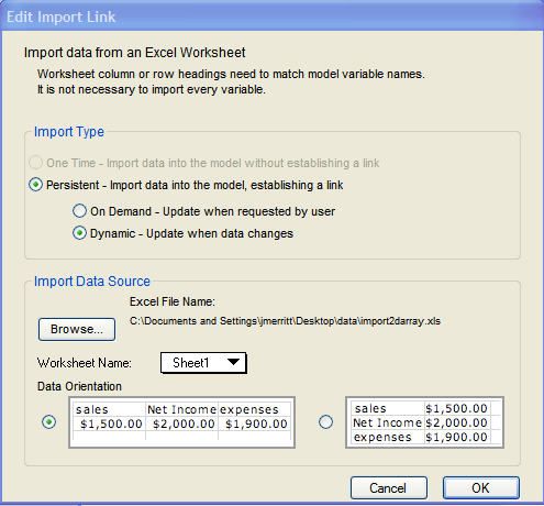
Open the Import Data dialog under the Edit Menu. Set up the link so that you are pointing to the spreadsheet you just created.
Select the Import Type you want and browse for the Excel file and worksheet you created. The data orientation you pick should match the orientation of the spreadsheet.
Once you click OK, a message will let you know if data was successfully imported or not.
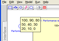
Now check to see that the data was imported by hovering over the arrayed variable.
It worked!! You’re good to go.

