What is Delta Time (DT)?
After reading Karim Chichakly’s recent post on Integration Methods and DT, I was reminded that delta time (DT) has always been a tricky modeling concept for me to grasp. Beginning modelers don’t usually need to think about changing DT since STELLA and iThink set it to a useful default value of 0.25. But once you progress with your modeling skills, you might consider the advantages and risks of playing with DT.

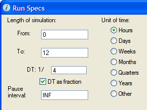
By definition, system dynamics models run over time and DT controls how frequently calculations are applied each unit of time. Think of it this way, if your model was a movie, then DT would indicate the time interval between still frames in the strip of movie film. For a simulation over a period of 12 hours, a DT of 1/4 (0.25) would give you a single frame every 15 minutes. Lowering the DT to 1/60 would give a frame every minute. The smaller the DT is, the higher the calculation frequency (1/DT).
Beware of the Extremes
A common tendency for modelers is to set the calculation frequency too high. Without really thinking too hard about it, more data seems to imply a higher quality model – just like more frames in movie film make for smoother motion. If your model calculates more data for every time unit, its behavior will begin to resemble the behavior of a smoothly continuous system. But a higher frequency of calculations can greatly slow down your model’s run performance and more data does not directly translate to a better simulation.
Beware of Discrete Event Models
Another situation where DT can often lead to unexpected behavior is with models that depend on discrete events. My eyes were opened to this when I attended one of isee’s workshops taught by Corey Peck and Steve Peterson of Lexidyne LLC.
One of the workshop exercises involved a simple model where the DT is set to the default 0.25, the inflow is set to a constant 10, and the outflow is set to flush out the stock’s contents as soon as it reaches 50. This is how the model’s structure and equations looked:

Stock = 0
inflow = 10
outflow = IF Stock >= 50 THEN 50 ELSE 0
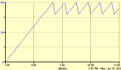
I would have expected the value of the stock to plunge to zero after it reached or exceeded 50, but this graph shows the resulting odd saw-tooth pattern.

The model ends up behaving like a skipping scratched record, in a perpetual state of never progressing far enough to reach the goal of zero. (Click here to download the model.)

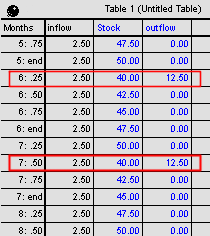
What is happening in the model? In the first DT after the stock’s value reaches exactly 50, the outflow sets itself to 50 in order to remove the contents from the stock. So far so good, but now the DT gotcha begins to occur. Since the outflow works over time, its value is always per time. To get the quantity of material that actually flowed, you must multiply the outflow value (or rate) by how long the material was flowing. When DT is set to 0.25, the material flows 0.25 time units each DT. Hence, the quantity of material removed from the stock is 50*0.25 = 12.50.
Suddenly we are in a situation where only 12.50 has been removed from the stock but the stock’s value is now less than 50. Since the stock is no longer greater than or equal to 50, the outflow sets itself back to 0 and never actually flushes out the full contents of the stock.
So what do we do? One solution to this problem would be to use the PULSE built-in to remove the full value from the stock. Here’s what the equation for the outflow would look like:
outflow = IF Stock >= 50 THEN PULSE(Stock) ELSE 0
(Note: This option will only work using Euler’s integration method.)
Further Reading
STELLA and iThink have great help documentation on DT. The general introduction provides a good explanation of how DT works. The more advanced DT Situations Requiring Special Care section focuses more on artifactual delays and the discrete model issues mentioned in this post. Delta time and resulting model behaviors are reminders that system dynamics models run over time, but they achieve this by applying numerous discrete calculations in order to simulate the smooth behavior of actual systems.