COVID-19: Modeling Distributions of Incubation and Recovery Times

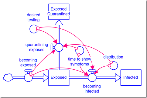
There is a flurry of models becoming available for the coronavirus pandemic we are in the midst of.  We at isee systems have issued our own, available here.  We’ve noticed a number of people use the canonical Susceptible-Exposed-Infected-Recovered (SEIR) model (in its simplest form):

We’ve used this same model, albeit with disaggregation of severity of infection and the population that has been tested.  We observed with our model that the simple first-order material delay used to model Exposed people becoming Infected and Infected people becoming Recovered is not appropriate for this situation and has a significant impact on the results.  We chose to use an infinite-order delay, but that also is not quite right.

When choosing the order of a delay, one should consider the distribution of times around the specified delay time.  An infinite-order delay will delay all material for exactly that amount.  However, lower-order delays will delay material according to a distribution.  The shape of that distribution can be discerned with a PULSE.  As you can see in the graph below, the first-order material delay releases a large fraction of material almost immediately.

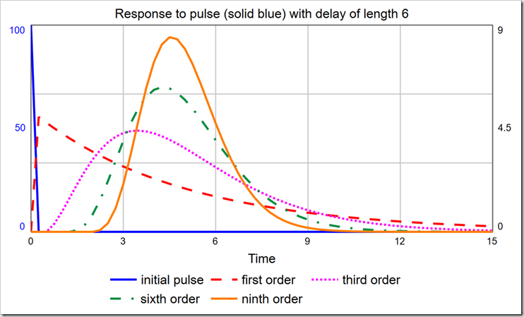With a delay time of six, the modes for the 1st-, 3rd-, 6th-, and 9th-order delays are, respectively:  DT (0.25), 3.5, 4.25, and 4.5.  It is certainly not true that the largest group of people who become Exposed move on to being Infected almost immediately (after one DT).  To correct this, we must use a higher-order material delay.  Notice the 3rd-, 6th-, and 9th-order delays are all skewed right (their peaks are not centered on the actual delay value, which is six, and they are asymmetric).  You can pick the order that most closely matches the actual distribution of, for example, time to show symptoms.  The latest data I saw said that the average time to show symptoms is 5 days, but many cases can be 14 or more days.  This indicates a long tail on the right side, making a 3rd- or a 6th-order more appropriate than a 9th-order.  It would be ideal, though, if we could experiment with different distributions just by changing the order.

Normally, we would explicitly expand the model to handle a higher-order delay.  However, consider that a 3rd-order delay requires three stocks, and a 6th-order requires six stocks, instead of just one.  This muddies up the diagram quite a bit and does not give us the flexibility to easily change the order because any change requires a change to the model structure.  The alternative is to use the DELAYN function, which allows you to specify the order of the delay as a parameter.  The problem with this approach is that you only have access to the output of the delay (a flow); you no longer have access to the contents of the stock.  In this application, we need to see how many people are Exposed and Infected.  In Business Dynamics, John Sterman proposes the following structure for this exact circumstance:

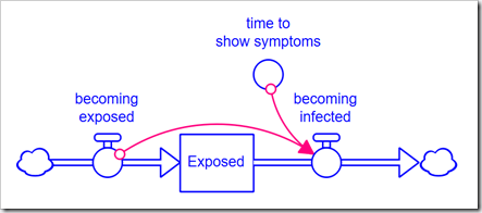Rather than formulate the outflow becoming infected as a draining process (based on the stock), it is formulated from the inflow using the equation, for example, for a 3rd-order delay:

DELAY3(becoming_exposed, time_to_show_symptoms, 0)

You can use DELAYN instead to specify the order, and therefore the distribution, you wish to use as a parameter.  This formulation works very well.  However, in this instance, we wish to model testing.  Testing will remove people from both Exposed and Infected (note that with COVID-19 people can be Infected and still be asymptomatic, so quarantining when symptoms appear is not sufficient).  This formulation breaks down when you have multiple outflows from a stock because everything entering the stock is assumed to exit the stock.

I tried to develop a simple formula to work around this problem.  Unfortunately, while the formula I developed more or less worked, it wasn’t robust.  That leaves us with doing it the hard way, i.e., explicitly expanding the structure.  The problems with this are, again, it is inflexible (we can’t change the order without changing the structure) and it makes the structure hard to interpret and understand.  The solution:  Create a general macro to handle this case.  We can first implement it in a module to test it and then move it to a macro when we’re happy with what we have.

Using arrays, I developed and tested the following module that allows the order to be specified as a parameter between 1 and 9 (the upper bound can easily be increased by changing the array dimension, Stage).  It has five inputs:  the inflow to the stock (input), the length of the delay (time to delay), the order of the delay (N), the initial value (initial), and the desired value for the second outflow (desired early exit).  It has two outputs:  the main outflow from the stock (out) and the second – in our model, testing positive – outflow (early out).  You can download the external module file here.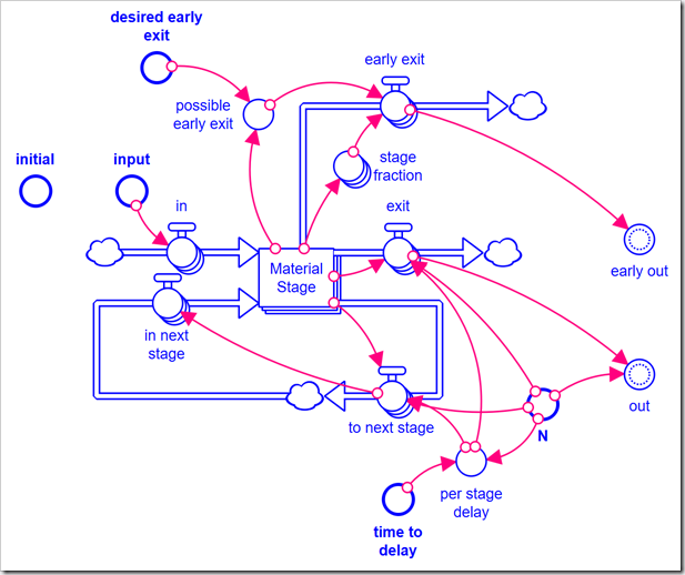This module is very specific to this application:  The second outflow is distributed across the intermediate delay stages based on each stock’s fraction of the total (stage fraction).  I.e., we assume a random draw from the Exposed population and this fraction is just the probability of drawing someone who has been in the Exposed stock for the time corresponding to that stage.

The relevant equations are, first, to transfer material between stages:

to_next_stage = IF Stage < N THEN Material_Stage/per_stage_delay ELSE 0
in_next_stage = to_next_stage[Stage – 1]

Then to get the output value:

exit = IF Stage = N THEN Material_Stage/per_stage_delay ELSE 0
out = exit[N]

The early exit is a little more complicated.  First, the desired flow is limited to the material available:

possible_early_exit = MIN(desired_early_exit, SUM(Material_Stage)/DT)

Note the contents of the stock are divided by DT because we are comparing to a flow (the alternative would be to multiply the flow by DT, but we want the flow value, not the stock value, in the end).  This is a discrete limit that one could argue should be continuous.  For example, one could argue that as the number of Exposed people falls below the capacity of testing, it is harder to find them and get them together for testing.  Using such an argument, you would use the fuzzy minimum construction (described in John Sterman’s Business Dynamics).  This is the most likely shape for a continuous formulation.  I did run tests with this alternate formulation and did not see any qualitative difference in the results.  Using an upper x-bound of 1.5 on the fuzzy minimum, I could not discern any difference.

Finally, we can calculate the amount that exits before the delay time:

stage_fraction = IF SUM(Material_Stage) <> 0
   THEN Material_Stage/SUM(Material_Stage) ELSE 0
early_exit = stage_fraction*possible_early_exit

Note again that stage fraction[Stage] is the probability of drawing a random person from that stage.

Testing this, it does all we hoped for and works for delay orders from 1 to 9, selected as a parameter as desired.  We could import this into any number of modules and use it many times in our model.  Ideally, though, we could put it in a macro and hide the messy computations and any module connections out of the way.  We have two problems in turning this into a macro:

1. Macros have only one output (they are invoked just like builtin functions).  This is easily resolved by creating two macros with identical parameters and structure but different outputs.
2. At this date, Stella^® does not support arrays in macros.  That means we have to unfold this formulation into many separate stocks.  We will turn our attention to this now.

In unfolding this from an array representation to an explicit one, one might be tempted to create a main chain of nine stocks.  This can work, but makes the formulation much more complicated (you either have to exit all the material at the correct stock based on N or only include the first N stocks in your sums).  It makes more sense to be more literal in the translation from the array, creating separate inflows and outflows for each stock and connecting the outflow of one stage to the inflow of the next stage, just as we did with the array.  Here are the first two stages (the rest follow the same pattern as stage 2):

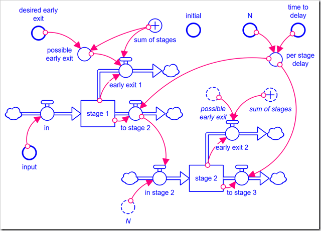Instead of having a separate stage fraction variable for each stage, I buried the formula in the respective early exit flows.  For example, the equation for early exit 2 is:

IF sum_of_stages <> 0 THEN possible_early_exit*stage_2/sum_of_stages ELSE 0

The variable sum of stages is just the sum of stocks stage 1 through stage 9.  The equation for the in stage 2 through in stage 9 have to stop the flow continuing down the chain once N stocks have been passed through.  The in stage 2 equation is:

IF N >= 2 THEN to_stage_2 ELSE 0

Stage 3 compares N against 3, stage 4 compares N against 4, etc.  Finding the value of early out is easy.  It just sums early exit 1 through early exit 9.  Finding the value of out is more complicated.  We have to explicitly check N to find the correct outflow:

IF N = 1
THEN to_stage_2
ELSE IF N = 2
THEN to_stage_3
ELSE IF N = 3
THEN to_stage_4
ELSE …

The last step is to place these in two macros.  I called one DELAYN2OUT and the other DELAYN2OUT2ND (to get the second outflow).  They both take the same parameters I listed for the array-based version – and in that order (and can be downloaded here).  Here is how I used them in my SEIR model:

The equation for becoming infected is:

DELAYN2OUT(becoming_exposed, time_to_show_symptoms, distribution,
   0, desired_testing)

The equation for quarantining exposed is the same except it used DELAYN2OUT2ND.  The entire model can be downloaded here.  A two things to note about this model:  First, I assume that all Infected people show symptoms and self-isolate.  This is not the case with COVID-19, but means the above macros are not used again here as the impact would be small.  Second, the next step would be to disaggregate by severity or age group.  This would then give you some people exiting Infected due to symptoms showing and others staying with no symptoms.  You would then need the above macros across Infected.  You could then also have different contact rates and different death rates for the different groups.