Building a Health Care Model Hierarchically
I recently had the pleasure of building a very large model of the health care system from many small discrete parts. I did this in a course on Health Care Dynamics taught by James Thompson at Worcester Polytechnic Institute. The design of the model is entirely Jim’s.
The most striking thing about this model to me is that it was created completely hierarchically. I have seen many large models broken into sectors which are conceptually all at the same level. I have seen other large models that are organized by feedback loops, which can at some times be large and unwieldy. But I had yet to see an example that is truly hierarchical, with an appropriate dynamic hypothesis at each level.
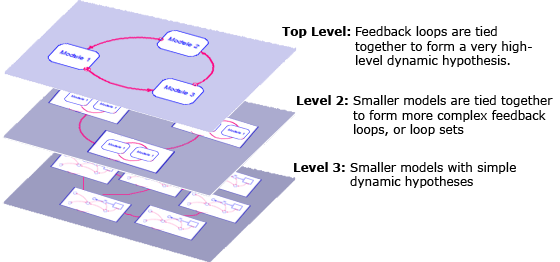
The model is three-levels deep. At the lowest level are models with very simple dynamic hypotheses. At the next level up, groups of these smaller models are tied together to form more complex feedback loops, or loop sets, comprising a higher-level dynamic hypothesis (this is the complexity most of the models I develop have). At the top-level, they are tied together to form a very high-level dynamic hypothesis. One of the very nice things about this is that each part of the model, which was built bottom-up, has already been tested in isolation or within its group before the whole model is tied together. All parts are in steady-state. In this way, we have built confidence in all of the parts of the model and now are only testing the broadest feedbacks.

Critics of this approach insist that delaying the connection of the broadest feedbacks until this late in the development of the model hides important dynamics that affect all parts. Not only is this considered risky, but the model does not generate results until the end. After this experience, I can’t agree with this point-of-view. There was very little risk in tying the pieces together at the end because they were well-formed pieces already rich in feedback, and (very important!) initialized in steady-state. While the model did not address some of the overarching issues until the end, careful testing of the pieces of the model added insight at many steps along the way and even gave hints about what might happen when those final feedbacks were put into place.
One of the key questions this model attempts to address is how to combat the rising costs of health care. The highest level dynamic hypothesis shows this to be exceedingly difficult because the processes in place at this level are all reinforcing loops:
The outer loop, R1, goes like this: As population grows, there is more demand for health services (thru physicians). As these services are used, more money is spent on technology (including pharmaceuticals), more money is devoted to research, and more causes of death are held in abeyance. This increases expected longevity, which increases the population. Of course, there must be physical limits to this (mustn’t there?), but it comes down to how much people are willing to pay to live a little longer.
The smaller loop, R2, goes like this: Better technology (new or improved treatments) itself drives more demand for health care services, which creates more research dollars, and thus more technology.
In other words, desire for longer lives and better treatments itself serves to drive up health care costs. This is a tough lesson.
The details are, of course, much more complicated than this. For example, at some point, and some would say we have already reached that point, we will hit diminishing returns. That is, we will have to spend far more money for a smaller incremental improvement in life expectancy. Will the market bear the costs of this research?
Moving down a level into the Physicians module, we find another dynamic hypothesis:
As the number of physician visits increase, the physician capacity in hours increases (note the number of physicians itself does not typically respond as limits are set by AMA policy). As the number of hours worked increases, physician prices increase. Higher prices lead to fewer visits. This is a simple balancing loop. When the visit rate falls sharply, this balancing loop operates slightly differently: As number of physician visits decrease, physicians have more free time to attend to each patient, lower their prices, and drive the visit rate back up both through lower prices and an increased frequency of visits.
Drilling down to the third and final level, we find this structure within Physician Visits:
This includes the effects of a managed care organization (MCO) trying to manage utilization rates of physician services (UM is utilization management). As the visit rate increases, the MCO works to reduce the visit rate. However, as the visit rate falls, patient satisfaction also falls and patients work to circumvent the MCO initiatives, thus bringing the visit rates up. There are thus two balancing loops working in opposition to each other. As you can easily imagine, they arrive at a compromise somewhere in the middle.
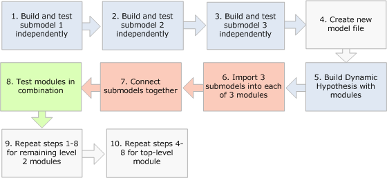
I have built a number of smaller models using modules and I have built them all from the top down. I draw out my dynamic hypothesis using modules and then drill-down into each module to flesh out its dynamics. Using Run by Module, I can test these modules in isolation and then in combination with others as they become available. I start with one model file and I end with one model file. I show this workflow below.

This model of the health care system was built from the bottom up. This process was therefore quite different. Each model at the lowest level was built and tested independently as its own model file. Once I was convinced a model was working properly, I would move onto the next. Once I had the pieces completed for a loop set of interacting models (for example, the contents of the Physicians module), I would create a new model file, create a sketch of the dynamic hypothesis at this higher level and then import the already working models into those modules. After connecting the variables across those modules, I could test different combinations of modules in that loop set.
Finally, when I had finished all loop sets, I created one more model file for the entire model. I drew the dynamic hypothesis for this model using modules and then imported the already working loop sets into the modules. I then only had to connect the variables across this level and test the various combinations of modules until I was satisfied the entire model was doing what it was supposed to do. I show this workflow below, assuming three submodels at the lowest level and a total of three levels.

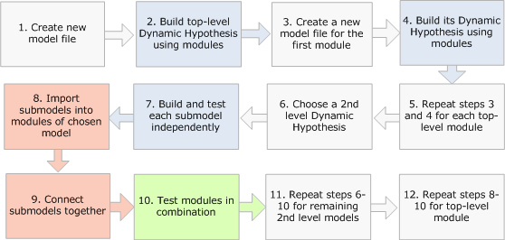
Of course, it was a great advantage that the model had already been designed and implemented once before by Jim Thompson. For such a large model, it would most often be disastrous to just start building at the bottom without knowing how it was going to tie together at the top. Because he did such an excellent job in partitioning this model, it worked out very well. I suggest, therefore, that a hybrid approach – both top-down and bottom-up – is more likely to succeed when starting a new project. In this case, the architecture gets worked out ahead of time in the form of dynamic hypotheses at each level. Then the smaller models can be built. Indeed, this really is the approach I followed because Jim had worked out the dynamic hypotheses at each level ahead of time for me. I show this workflow below, assuming three levels.
