Spatial Modeling in Two Dimensions

Editor’s Note:  This is part 2 of a 3-part series on spatial modeling in iThink and STELLA.  Part 1 is available here.  Part 3 is available here.

Last time, we explored spatial modeling using the one-dimensional diffusion problem as an example.  Many spatial applications, however, require two dimensional formulations.  As an extension, we will now explore the two-dimensional diffusion problem.  Instead of a one-meter metal bar with constant heat applied at its ends, the two-dimensional diffusion problem looks at the response of a one-meter by one-meter metal plate with constant heat applied to its center.  We then watch the heat diffuse across the plate.

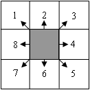
At first blush, one might think the two-dimensional case is much more difficult than the one-dimensional case.  In particular, if a grid is superimposed over the plate, each finite element on the plate has eight neighbors, as shown below.  It is tempting, therefore, to consider radiating heat in each of these eight directions.

However, without looking at the two-dimensional diffusion equations, if we consider just the physical layout of this system, the four corners of the finite element only touch the four corner neighbors (1, 3, 5, and 7) at one point.  In contrast, the four sides of the finite element are shared with each of its four immediate neighbors (2, 4, 6, and 8).  This suggests that heat only radiates to (and from) these four neighbors, not all eight.  In fact, if we examine the two-dimensional diffusion equation, we find that there are only component contributions in the x– and the y-directions.  There are no contributions on the diagonal (which would appear in the equation as ∂²u/∂x∂y and ∂²u/∂y∂x terms).

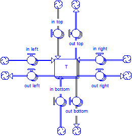
Intuitively, then, we have a finite element that is very similar to the one-dimensional case.  We only need to add corresponding flows in the y-direction.  This leads to the following model with the individual finite elements arrayed.

The array T is now two-dimensional, in x and in y.  In addition, dx can differ from dy, so the diffusion constant C must be broken down into its constituent parts C_x = k/dx² and C_y = k/dy².  This leads to the following set of equations for the radiant flows through the plate:

in left = Cx*T[X – 1, Y]                               in top = Cy*T[X, Y – 1]
out left = Cx*T[X, Y]                                  out top = Cy*T[X, Y]
out right = Cx*T[X, Y]                              out bottom = Cy*T[X, Y]
in right = Cx*T[X + 1, Y]                          in right = Cy*T[X, Y + 1]

X and Y are dimension names for the elements in the x– and ­y-directions, respectively.

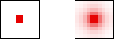
Using isee Spatial Map, it is possible to view the results of this diffusion across two dimensions.  Spatial Map displays an array as a one-dimensional or two-dimensional grid (depending on the array).  Each cell in the grid is filled with a color corresponding to the value in the corresponding cell of the array.  Below are two spatial maps.  The one on the left shows the initial conditions of the metal plate.  Note that heat only appears in the center of the plate, where it is being externally applied.  The map on the right shows the distribution of heat across the plate at the end of a six-minute simulation.

The model is available here:  2d-diffusion.  It is already configured to use isee Spatial Map.  In the final installment of this 3-part series, I will describe how to set up isee Spatial Map.