Integration Methods and DT

The simulation engine underlying STELLA® and iThink® uses numerical integration.  Numerical integration differs from the integration you may have learned in Calculus in that it uses algorithms that approximate the solution to the integration.  The two approximations currently available are known as Euler’s method and the Runge-Kutta method.  All algorithms require a finite value for DT, the integration step-size, rather than the infinitesimally small value used in Calculus.  On the surface, it may seem that the smaller DT is, the more accurate the results, but this turns out not to be true.

Compound Interest:  Euler’s Method over Runge-Kutta

To introduce Euler’s method, let’s take a look at the simple problem of compound interest.  If we have $100 that we invest at 10% (or 0.1) compounded annually, we can calculate the interest after N years by adding in the interest each year and recalculating:

1st year:  interest = $1000 × 0.1 = $100; Balance = 1000 + 100 = $1100
2nd year: interest = $1100 × 0.1 = $110; Balance = 1100 + 110 = $1210
3rd year:  interest = $1210 × 0.1 = $121; Balance = 1210 + 121 = $1331

And so on up to year N.  We have just seen the essence of how Euler’s method works.  It calculates the new change in the stock for this DT (in this case, interest) and then adds that to the previous value of the stock (Balance) to get the new value of the stock.  In this example, DT = 1 year.

By noticing we always add the existing balance in, we can instead just multiply the previous year’s balance by 1 + rate = 1 + 0.1 = 1.1:

1st year:  Balance = $1000 × 1.1 = $1100
2nd year: Balance = $1100 × 1.1 = $1210
3rd year:  Balance = $1210 × 1.1 = $1331

And so on up to year N. We can further generalize by noticing we are multiplying by 1.1 N times and thus arrive at the compound interest formula:

Balance = Initial_Balance*(1 + rate)^N

Checking this, we find our Balance at the end of year 3 is 1000*1.1^3 = $1331.  In the general case of the formula, rate is the fractional interest rate per compounding period and N is the number of compounding periods (an integer).  In our example, the compounding period is one year, so rate is the annual fractional interest rate and N is the number of years.  However, if interest is compounded quarterly (four times a year), the interest rate has to be adjusted to a per quarter rate by dividing by 4 (so rate = 0.1/4 = 0.025) and N must be expressed as the number of quarters (N = number of years*4 = 3*4 = 12 for the end of year 3).  We can use this formula in our model to test the accuracy of Euler’s method.  Note that for quarterly compounding, we would set DT = 1/4 = 0.25 years.

To explore the differences between Euler’s and Runge-Kutta, the following structure will be used for all of the examples in this post.  This structure models the compound interest problem outlined above.

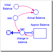
The equations change for each example and can be seen in the individual model files (accessed by clicking here).  For this example, the actual value is calculated using the compound interest formula, Initial_Balance*(1 + rate)^TIME.  The approximated value is calculated by integrating rate*Approx_Balance (into Approx_Balance).

In addition to the actual and approximate values, three errors are also calculated across the model run:  the maximum absolute error, the maximum relative error, and the root-mean-squared error (RMSE).  The absolute error is:

ABS(Actual_Balance – Approx_Balance)

The relative error is:

absolute_error/ABS(Actual_Balance)

and is usually expressed as a percentage.  The RMSE is found by averaging the values of the absolute error squared, and then taking the square root of that average.

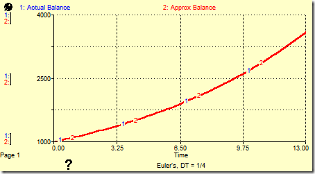
Running this model under Euler’s method leads to the behavior shown in the following graph.  As expected, Euler’s method tracks this function perfectly.  All three errors are essentially zero.

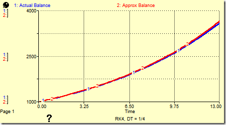
However, changing the integration method to Runge-Kutta 4 (known as RK4) does not give a good approximation (see graph below).  The relative error is 1.6%, the absolute error is $56 and the RMSE is $26, all rather large for RK4.  DT must be reduced a factor of 32, to 1/128, in order to bring the errors below 0.1% (0.001).

Continuous Compounding:  Runge-Kutta over Euler’s Method

Our friend Euler was a busy mathematician.  He is also famous for discovering the formula for continuously compounding interest.  If you increase the frequency of compounding from once a year to once a month to once a day (what most banks do now and called “daily compounding”) to once a second and so on until you are compounding every infinitesimally small instant (which should remind you of the dt from Calculus), the compound interest formula becomes:

Balance = Initial_Balance*e^(rate*time)

where e ≈ 2.718281828 is Euler’s number, rate is the annual fractional interest rate, and time is the number of years that have passed (a real number).  Using continuous compounding, our Balance at the end of year 3 is 1000*e^(0.1*3) ≈ $1350, $8 more than with annual compounding.

This function is known as continuous function, which, in layman’s terms, means its value smoothly changes with time, rather than experiencing jumps or gaps.  [Note the compound interest formula given in the first section is not continuous; since N must be an integer, this function only exists at integer values.]  While Euler’s method does not depend on a function being continuous, it does introduce an error proportional to DT when trying to integrate these equations (called truncation error).  Thus, the only way to reduce these errors is to reduce DT, requiring more computations.  Unfortunately, this only works up to a point.  Below that point, errors increase again due to round-off error in the computer’s finite representation of floating point values.

The graph below shows the effect of using Euler’s method to calculate continuously compounding interest.  Note it does not follow the actual curve, calculated with the EXP function, very well.  The relative error is 1.6%, the maximum error is $56, and the RMSE is $25.  If we cut DT in half, to 1/8, the errors also cut in half as we expect, to 0.8%, $29, and $13, respectively.  This will continue until DT reaches the limit of the machine’s representation, which is approximately 1/2048 for single-precision floating point numbers and 1/67,108,864 (1/2^26) for double-precision floating point numbers (note STELLA and iThink always use double-precision).  After this point, errors will increase again.  Note these values are theoretical; your mileage will vary.

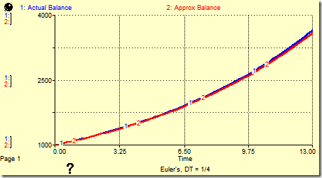
There is a better solution than reducing DT.  The Runge-Kutta integration method assumes a continuous function and takes steps to follow such a function very closely.  Because it uses a weighted average of values across each DT-interval, it does not perform well with discontinuous functions, i.e., functions that have gaps or sharp changes, such as that produced with the STEP and PULSE functions (however, STELLA and iThink compensate for this so that these functions still perform correctly under Runge-Kutta).  Leaving DT at 0.25 and changing the integration method to RK4 produces the following graph, with the largest relative error being 0.0077%, the largest absolute error being $0.27 and the RMSE being $0.14.  To achieve this level of accuracy with Euler’s method, it is necessary to reduce DT to 1/1024.

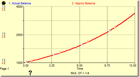
The number after the RK is the order of the integration method.  Typically, but not always, higher-order methods will give smaller errors.  Euler’s method is a first-order method and RK4 is a fourth-order method.  Note, however, that Euler’s outperformed RK4 in the first example.  STELLA and iThink also provide a second-order method, Runge-Kutta 2 (RK2), which is a compromise between Euler’s and RK4; with the speed of today’s computers, it is no longer necessary to use and remains only for backward-compatibility.

Oscillations:  The Case for Runge-Kutta

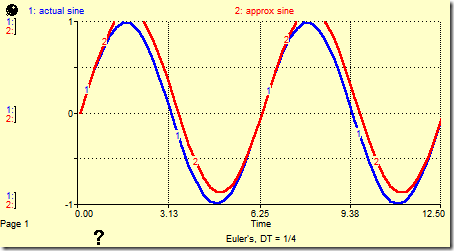
Oscillations represent one area where RK4 really shines.  The following graph shows the results of using Euler’s method to integrate the sine function with DT = 0.25.  Notice it misses horribly.  The resulting function is clearly outside the range of the sine function [-1, 1].  The maximum absolute error is 0.25 and the RMSE is 0.15.  However, the maximum relative error is 340%!

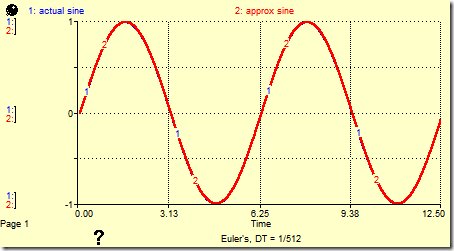
Reducing DT by a factor of 128 to 1/512 helps somewhat (below).  The maximum absolute error reduces to 0.0020 and the RMSE to 0.0012, but the maximum relative error only decreases to 200%.

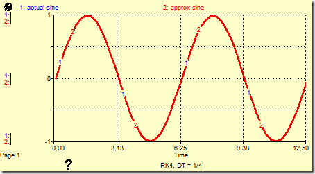
On the other hand, if we leave DT = 0.25 and change the integration method to RK4, it calculates the sine function quite well, with a maximum absolute error of only 0.0078 and an RMSE of 0.0045.  The maximum relative error is also acceptable at 2.2%.  Cutting DT in half to 1/8 reduces the maximum relative error an order of magnitude, to 0.34%.

Guidelines for DT

DT should initially be set to one-half of the smallest time constant in your model.  This minimal value, according to Nyquist’s Sampling Theorem, avoids undersampling your values.  [Undersampling means looking at your signal so infrequently that you distort the signal, or, more to the point, do not have enough information to reconstruct it.  For example, in the sine wave above, evaluating it every π will make you think you have a straight line at the origin, since all you will see are the zeroes.]

Finding the smallest time constant can be tricky.  They often appear in compounding or in draining processes.  For example, in the first two examples, the interest rate is the reciprocal of the time constant (it always appears in the divisor).  Thus, the time constant for this compounding formula is 10.  This suggests DT could start at 5, but there are other constraints.  In fact, we wish to compound every quarter, so DT must be set to 1/4.

Run the model with your chosen DT.  Then cut DT in half and try again.  If the results change, cut DT in half and try again.  If they do not change, the previously chosen DT is likely fine.

Whenever possible, choose a value of DT that is a power of 2 (1, 1/2, 1/4, 1/8, 1/16, … or 1, 0.5, 0.25, 0.125, 0.0625, …).  This is because most other fractions, for example 1/10, are repeating decimals in base-2 and so cannot be accurately represented on the computer.  Obviously if your problem requires you to use a DT of 1/7, in weekly simulations for example, do so, but understand that adding 1/7 seven times will not equal one.  There are also other cases where you might need to use a DT that is not a power of 2.  If your smallest time constant is 1/52, for example, choosing the closest power of 2 to (1/52)/2 = 1/104, which is 1/128, would be disastrous.  Your time constant would then be 1/64 sometimes and 1/32 other times, not at all close to what you need.  Make sure you can represent your smallest time constants as a multiple of whatever DT you choose.

Guidelines for Integration Method

Changing DT is often not sufficient.  Your system may exhibit instabilities or wild oscillations caused by the errors in Euler’s method.  It is therefore also wise to always run the model in Euler’s and then in RK4.  If there is a difference, stick with RK4 and proceed to test DT.

Euler’s method is noticeably faster than RK4 and works fine in many situations.  A system that has linear relationships and uses exponential functions that are not based on Euler’s number will work fine using Euler’s method.  For qualitative results, Euler’s will work well in a broad variety of situations.  Euler’s is also the preferred method when you are using discontinuous or discrete functions (but note the discrete functions in STELLA and iThink are Runge-Kutta-aware and should work reasonably well under RK4).

Any continuous system that is based on exponential functions using Euler’s number as a base, and this includes trigonometric functions, oscillations, and logistic functions, will be better served by RK4.  In these cases, you should generally use this method from the start.

There is one additional type of system you may run into that neither of these methods will solve very well:  stiff systems.  In simple terms, a stiff system is one that has time constants of wildly different magnitudes, for example, 0.005 and 10,000.  The smaller time constant suggests a DT of 0.0025 which is far too small for the part of the system with a time constant of 10,000.  It is best to reframe your problem to avoid these situations when possible.  For example, when simulating such a system, the part of the system with a time constant of 10,000 can often be considered constant over a shorter period of interest.  Over long periods of interest, it is often possible to aggregate the behavior of the part of the system with the shorter time constant, using averages instead of exact values.

Note:  The integration method and DT are both set in the Run Specs, accessible from the Run menu.  Additional information can be found in the chapter on DT in the Technical Documentation.