Using PEST to Calibrate Models

There are times when it is helpful to calibrate, or fit, your model to historical data. This capability is not built into the iThink/STELLA program, but it is possible to interface to external programs to accomplish this task. One generally available program to calibrate models is PEST, available freely from www.pesthomepage.org. In this blog post, I will demonstrate how to calibrate a simple STELLA model using PEST on Windows. Note that this method relies on the Windows command line interface added in version 9.1.2 and will not work on the Macintosh. The export to comma-separated value (CSV) file feature, added in version 9.1.2, is also used.

The model and all files associated with its calibration are available by clicking here.

The Model

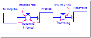
The model being used is the simple SIR model first presented in my blog post Limits to Growth. The model is shown again below. There are two parameters: infection rate and recovery rate. Technically, the initial value for the Susceptible stock is also a parameter. However, since this is a conserved system, we can make an excellent guess as to its value and do not need to calibrate it.

The Data Set

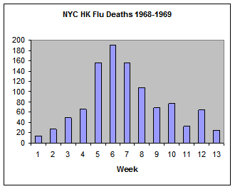
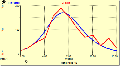
We will calibrate this model to two data sets. The first is the number of weekly deaths caused by the Hong Kong flu in New York City over the winter of 1968-1969 (below).

The second is the number of weekly deaths per thousand people in the UK due to the Spanish flu (H1N1) in the winter of 1918-1919 (shown later).

In both cases, I am using the number of deaths as a proxy for the number of people infected, which we do not know. This is reasonable because the number of deaths is directly proportional to the number of infected individuals. If we knew the constant of proportionality, we could multiply the deaths by this constant to get the number of people infected.

 

Preparing the Model

The original model ran from 0 to 40 days. This needs to be changed to match the data, i.e., to 1 to 13 weeks. Changing this will force us to change the parameter values also, as described below.

The initial values of Susceptible and Infected must be changed to match the data set. The total number of people in the model should match the total population in the data. Summing the Hong Kong flu data set gives a population of 1035 people. The initial value for Infected is just the first reported value, 14. That leaves 1021 people that are Susceptible.

If you run the model using the original parameter values, you will find the infection is spreading far too quickly. To improve the chances of the calibration succeeding, it is necessary to adjust the parameters so that the results are in the ballpark of the historical data. To do this, it is useful to paste the historical data into a graphical function (called data in this model) and graph it alongside the model output. I first reduced the infection rate from 0.005 to 0.0015 and then adjusted recovery rate from 0.25 to 0.5 to get a closer fit to the data.

The model must also be modified to persistently import its parameters and export the time series we wish to fit to the historical data. The import sheet is most easily set up by creating an empty CSV file, exporting “all model variables” and “One set of values” to this file, and then removing the variables that are not needed from this file. The file can also be built manually. The final file, input.csv, looks like this:

infection rate,recovery rate
0.0015,0.5

You will also need to create an empty file called output.csv for the exported data.

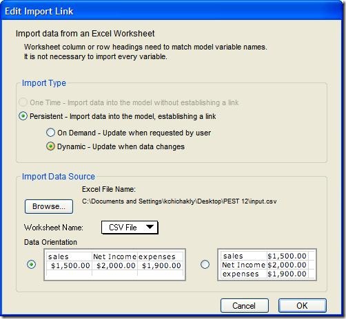
Set up the import by choosing Edit->Import Data… and entering the settings shown below:

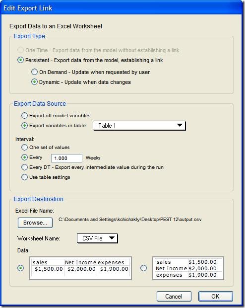
Add a table, called Table 1, to the model and add the stock Infected to the table. Set up the export by choosing Edit->Export Data… and entering the settings shown below. Note the “Use table settings” option is not used. This option cannot be used for calibration as it will restrict to precision of the output to match the table.

Save the model. It is ready to be calibrated.

Setting up PEST

PEST is a very powerful program. This post will only touch on the simplest capabilities that it provides. For more details and for more complex uses, consult the PEST manual.

PEST requires three text input files:

• The template file (.tpl), which tells it how to write the parameters to the model input file (input.csv in our case).
• The instruction file (.ins), which tells it how to read the data from the model output file (output.csv in our case).
• The control file (.pst), which tells PEST what to do.

Creating the Template File

This is the simplest file to create, as it only requires replacing data values in the model input file with markers so PEST can insert the parameter values it chooses.

Open the model input file, input.csv, in a text editor. Add the following line to the top of the file:

ptf #

This tells PEST this is a template file and that parameter fields, including the parameter name, will be surrounded by pound signs (#).

Replace each parameter value in the file with a short alphanumeric name for that parameter, surrounded by #s. Add any additional spaces that are necessary to make each field 13 characters long, including the pound signs. Using 13-character field widths, which is the maximum precision in single-precision floating point, is absolutely necessary to make certain the calibration succeeds (see end note about precision).

Save this file as input.tpl. The final file should look like this:

ptf #
infection rate,recovery rate
#infectrate #,#recoverrate#

Creating the Instruction File

The instruction file contains a set of instructions that PEST can follow to extract the model-generated data that corresponds to the historical data from the model output file. The model output file is a CSV file that has a header line followed by 13 lines, one for each week in the model run. Each of the 13 lines contains two numbers separated by a comma. The first value on each line is the week number and the second is the number of people who have been infected.

The contents of the instruction file, output.ins, appear below:

pif @
l2 @,@ !infected1!
l1 @,@ !infected2!
l1 @,@ !infected3!
l1 @,@ !infected4!
l1 @,@ !infected5!
l1 @,@ !infected6!
l1 @,@ !infected7!
l1 @,@ !infected8!
l1 @,@ !infected9!
l1 @,@ !infected10!
l1 @,@ !infected11!
l1 @,@ !infected12!
l1 @,@ !infected13!

The first line tells PEST that this is an instruction file and that the at-sign (@) will be used to delimit search keys. Each succeeding line tells PEST how to read the model output file, output.csv.

Each instruction line starts with a lowercase L, the PEST command to skip to the beginning of the Nth following line. The number one (1) is used to move to the start of the next line (interpreted as the start of the first line when at the beginning of the file), while larger numbers skip over an additional N – 1 lines. Thus, the “l2” in the first command, moves to the start of the second line in the file, skipping over the header. Each additional command uses “l1” to move to the start of the next line.

On every single line, it is necessary to skip to the second field (Infected), as we do not care about the week number. Surrounding the comma in at-signs (@,@) tells PEST to move to the next comma it finds (which will be the first comma on the line in all cases shown here). The exclamation points (!) delimit the name of the observation (historical data point) that corresponds to the data after the comma (called observation names in PEST). Note that each value of a time-series requires a unique observation name and that each observation name cannot be longer than 20 characters. In this case, there are 13 values, one for each week, in our historical data and our model-generated data, so the variables are named infected1 thru infected13.

In many cases, there will be far more data values that need to be assigned names. The instructions in this file, including the ever-incrementing names, can be quickly created in some text editors and also in Excel. The following formula can be pasted into cell A1 of Excel and filled down as far as necessary to create the proper instructions:

=CONCATENATE(“l1 @,@ !infected”, ROW(A1), “!”)

The above instruction names uses the name infected as the root of all observation names. Make sure to change this name in the above formula to match the variable name in your model. After you copy the text generated by Excel into your instruction file, make sure to change the first command so that it begins with “l2” rather than “l1”. If you fail to do this, PEST will not skip over the header in output.csv and will abort when it tries to read numeric values from the text that appears there.

There will also be cases where it is desirable to calibrate to multiple pieces of data. In this case, the commands in the instruction file will have to be modified to include the additional data. For example, if there is a second historical time series Treated and Treated appears after Infected in the model output file, each command would change to (using the fifth value as an example):

l1 @,@ !infected5! @,@ !treated5!

Creating the Control File

The control file contains a number of PEST parameters, the historical data, the command to run the model, and the names of the other files needed by PEST. It is a difficult file to create on your own. Luckily, PEST provides some command line tools to help. In particular, PESTGEN will generate the control file (with default settings) from two simpler text files:

• The parameter file (.par), which lists the input parameters to the model
• The observations file (.obf), which lists the historical time series; INSCHEK can generate this from the model output file and the instruction file Both files are fixed-format, which means the field widths and alignment must be properly respected. It is easiest to create the parameter file by editing an existing parameter file (PEST outputs a parameter file containing the final parameter values at the end of a calibration; the file used for this calibration is also included with the model).

The parameter file for this model, hkflu.par, appears below.

  single point
    infectrate    1.5000000E-03     1.000000         0.000000
   recoverrate    0.5000000         1.000000         0.000000

The first line tells PEST to use single-precision floating point and to always include the decimal point when writing parameters to the model input file. The file then contains one line for each input parameter.

Each line starts with the name of the input parameter, as it appears in the template file, right-justified. This is followed by the initial value of that parameter, a scale factor (normally one) and an offset (normally zero). To add additional parameters, copy and paste the lines and make sure the columns line up with the existing lines.

The observations file contains all of the observation names with the historical data values for each. The command line tool INSCHEK, which comes with PEST, will generate this file by merging the observation names in the instruction file with data in a file formatted the same as the model output file. The instruction file has already been created. To complete this process, copy and paste the historical data into the second column (Infected) of the model output file, output.csv, and save it. Open the Windows command prompt window by choosing “Command Prompt” under All Programs->Accessories. Make sure to change the current directory to the directory containing your model and your PEST files. This is easily done by type “cd ” (the ending space is necessary) and then dragging the folder icon in the address field of the Windows Explorer window for that folder onto the command window. Reselect the command window and press Enter. The directory is now set. Now type:

inschek output.ins

Note that inschek will need to be preceded by the path to the PEST directory if you have not added the PEST directory to your PATH environment variable. This command will verify there are no syntax errors in your instruction file. If you get any errors, correct them and check again. Continue until there are no errors reported. Then type:

inschek output.ins output.csv

This will create the observations file, output.obf, from the data you pasted into output.csv.

It is now possible to create the control file, hkflu.pst. Type:

pestgen hkflu hkflu.par output.obf

If there are errors reported in the parameter file, fix them and try again. This command generates a default control file for case hkflu (short for Hong Kong flu – you can name it anything you want) with your parameter values and historical data. This file will require some editing before PEST can be run.

Editing the Control File

The generated file looks like this (to view, right-click on hkflu.pst, choose “Open With…”, and select WordPad):

pcf
* control data
restart  estimation
    2    13     2     0     1
    1     1 single point   1   0   0
  5.0   2.0   0.3  0.03    10
  3.0   3.0 0.001
  0.1
   30  0.01     3     3  0.01     3
    1     1     1
* parameter groups
infectrate   relative 0.01  0.0  switch  2.0 parabolic
recoverrate  relative 0.01  0.0  switch  2.0 parabolic
* parameter data
infectrate   none relative   1.500000E-03  -1.000000E+10   1.000000E+10
 infectrate     1.0000        0.0000      1
recoverrate  none relative   0.500000      -1.000000E+10   1.000000E+10
 recoverrate     1.0000        0.0000      1
* observation groups
obsgroup
* observation data
infected1      14.0000      1.0  obsgroup
infected2      28.0000      1.0  obsgroup
infected3      50.0000      1.0  obsgroup
infected4      66.0000      1.0  obsgroup
infected5      156.000      1.0  obsgroup
infected6      190.000      1.0  obsgroup
infected7      156.000      1.0  obsgroup
infected8      108.000      1.0  obsgroup
infected9      68.0000      1.0  obsgroup
infected10     77.0000      1.0  obsgroup
infected11     33.0000      1.0  obsgroup
infected12     65.0000      1.0  obsgroup
infected13     24.0000      1.0  obsgroup
* model command line
model
* model input/output
model.tpl  model.inp
model.ins  model.out
* prior information

This is also a fixed-format file, so you need to be careful when editing it. Luckily, only a few things need to be edited.

The “pcf” at the top of the file tells PEST this is a control file. The control data section sets a number of parameters that can stay the way they are unless the calibration does not work (in which case, you will need to dig deeply into the PEST manual to figure out what to change and how to change it). The parameter groups section, the observation groups section, and the observation data sections will not require any changes. However, the parameter data section needs to be adjusted and both the model command line and model input/output need to be specified.

For each parameter under parameter data, you must decide whether the changes made by PEST to the parameter will be relative (i.e., additive – the default), or factor (i.e., multiplicative). There are advantages and disadvantages to each, however, for a STELLA model, this simple guideline should help: change all time constants, rates, and multipliers to factor. In the SIR model, both variables are rates, so the word “relative” must be replaced with “factor ”. Note the two extra spaces after “factor”; the new text must completely fill the space formerly occupied by “relative”.

The default domain for each parameter is set to -1.0e10 to 1.0e10. You are likely to have better information (especially if it is a multiplier) and should enter it here in place of those numbers. I restricted the domain of infectrate to between 0.0001 and 0.01 and that of recoverrate to between 0.01 and 1.0. This was based on both my knowledge of these variables and some simple experiments I ran. The domains for these parameters could be much wider, as long as they stay above zero in both cases. This leads to the following changed lines (truncated after limits):

infectrate   none factor     1.500000E-03   1.000000E-04   1.000000E-02 …
recoverrate  none factor     0.250000       1.000000E-02   1.000000E+00 …

The model command line is changed to:

run.bat

The batch file run.bat contains commands to create the model output file and to run the STELLA SIR.stm model:

@echo off
echo > output.csv
start /min /wait “” “C:\Program Files\isee systems\STELLA 9.1.4\STELLA” -r SIR.stm

If STELLA was not installed to the default directory shown in the above command, run.bat will need to be edited to contain the correct path to STELLA.  The model output file needs to be recreated in the batch file (using echo) because PEST deletes the model output file before running the model.

Finally, the model input/output section was changed to name the template, model input, instruction, and model output files. Note these are not fixed-width fields.

input.tpl  input.csv
output.ins output.csv

Running PEST

Before running PEST, it is a good idea to verify that all of the input files are valid. This is accomplished with PESTCHEK:

pestchek hkflu

Fix any errors that are reported and repeat until all errors are gone. Note that PESTCHEK does not require the case name (hkflu) to be specified. Without the name, it will find all case names in the current directory (by searching for PEST control files) and check them all.

Finally, start the calibration process with:

pest hkflu

PEST will run until it detects no further changes or cannot proceed. Each iteration, it will report a value named phi. This is the sum of the squared residuals and should be decreasing each iteration. If PEST succeeds, the model input file will contain the best parameter values found and the model output file will contain the results obtained with those parameter values.

PEST outputs a number of files as well. As already discussed, the parameter file (.par) will be updated (or created) to contain the final successful parameter values. The run details file (.rec) will contain a log of the search, including parameter values tried and their relative success, as well as the final results compared to the historical data, with residuals. The 95% confidence interval for the parameters is also given. A number of other files are generated by PEST. See the PEST manual for further details.

The results of running PEST with this model and these initial parameters are shown in the graph below. The final parameter settings discovered by PEST were infection rate = 0.0015766646 and recovery rate = 0.82166505, with a final error (phi) of 4785.7 (compared to 773,059 with the original parameters).

Changing the Data Set

Shown below is the number of weekly deaths per thousand people in the UK due to the Spanish flu (H1N1) in the winter of 1918-1919.

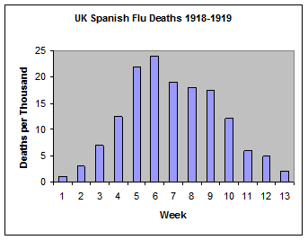
To calibrate to this data set, it is necessary to change the initial values of the Susceptible and Infected stocks in the model. The historical data values in the PEST control file must also be changed.

The initial value of Infected is, again, the first data value (1 in this case). The initial value of Susceptible is, again, the remaining population (148). The model SIR2.stm contains these changed settings, as well as the new historical data set.

While it is relatively easy to regenerate and edit the PEST control file, it is just as easy to edit the few historical values. Control file spflu.pst contains the new dataset. It also uses run2.bat to run SIR2.stm instead of SIR.stm. Type:

pest spflu

Although it takes some time, the calibration almost succeeds using the same starting parameters as those for the Hong Kong flu. It fails in the end because the domain of infection rate is too narrow; infection rate gets stuck at 0.01. It is important to note that PEST reported success in this case. Looking at the graph in STELLA, however, made it clear that it only came close, while looking at the chosen parameters showed the boundary was reached. Changing the maximum value to 0.1 in spflu.pst fixed that problem. The final results are shown below.

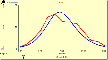
This was generated with infection rate = 0.012101631 and recovery rate = 0.89054160. The error decreased from 2233.8 at the start to 110.6 with these parameters.

Troubleshooting PEST

Chapter five of the PEST User Manual includes a detailed troubleshooting section titled “If PEST Won’t Optimize.” If PEST is not changing parameters or not succeeding, this section will help you discover why.

Troubleshooting Data

In the examples used in this post, the model-generated data was one-to-one with the historical data. In many cases, data is not collected at a set frequency, does not coincide in time with model-generated data, and there are missing data points. While this was not covered in this example, PEST is capable of dealing with these cases. Missing data points can be handled by using !dum! as a placeholder in the instruction file (or additional lines can be skipped between points). PEST can also interpolate the model-generated data to match it in time to the historical data. Refer to the PEST manual for instructions to handle these cases.

End Note (about precision): While STELLA and iThink use double-precision for its calculations and PEST supports double-precision output, it is not possible to directly interface to PEST in double-precision mode as PEST outputs exponentials using “D” instead of “E” when in double-precision mode (as FORTRAN does). Such non-standard numeric formats cannot be read by STELLA. Double-precision can be used if necessary by adding a preprocessor to convert those “D”s in the model input file to “E”s before running STELLA and by adding a post-processor after running STELLA to change the “E”s output by STELLA to “D”s. Each parameter should also be given a field that is 23 characters wide, instead of 13, in the template file. Most applications will not need to use double-precision.