Calibration in Stella®

This is the first of a three-part series on calibration and optimization. The second part can be accessed here. The third part can be accessed here.

Several years ago, I wrote a post that showed how to calibrate Stella and iThink® models using PEST, a third-party calibration tool (Using PEST to Calibrate Models). Starting with version 1.5, Stella Professional and Stella Architect have optimization built in. Since calibration is a special case of optimization, we can also use this feature to calibrate models (but stay tuned: calibration will be added as its own feature in the not too distant future). Let’s review the problem that was calibrated using PEST in that post and then configure the optimization to calibrate it within Stella.

The Model

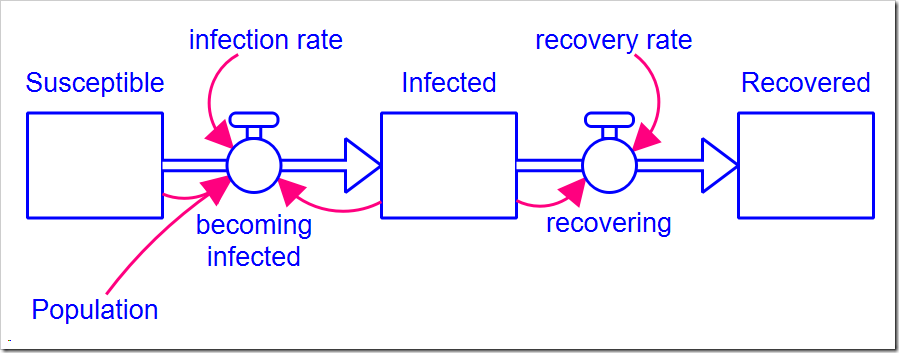
The model is a simple SIR model first presented in my blog post Limits to Growth and shown below (this version with all the optimization settings can be downloaded here). There are two parameters: infection rate and recovery rate. The Population size and the initial number of Infected people are also model parameters, but do not need to be calibrated (presumably, we know the population and the data tells us the initial number of infected people).

The Data Set

We will calibrate this model to the data set of the number of weekly deaths caused by the Hong Kong flu in New York City over the winter of 1968-1969 (below).

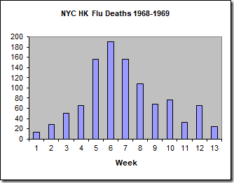
Here, I am using the number of deaths as a proxy for the number of people infected, which we do not know. This is reasonable because the number of deaths is directly proportional to the number of infected individuals. For this specific outbreak, less than 0.5% of infected people died, so we could multiply these numbers by 200 (1/0.005) to approximate the number of people infected. As I did not do this for the PEST calibration and wish to compare the results, I will not do this here either.

Calibration

To calibrate the model, we need to pick a metric that we will use to measure goodness of fit. Typically, we minimize this metric, which is…an optimization problem. There are a number of metrics available. e.g., root mean square error (RMSE), relative squared error (RSE), mean absolute error (MAE), relative absolute error (RAE), and the coefficient of determination (R², which you would maximize instead of minimize). It would be useful to compare these results to the earlier results from PEST, so we will use the sum of squares error (SSE, a component of R²), which PEST calls phi.  It is simply the sum of the squares of differences between the observed (data) values and the model values. We will need to add some structure to our model to calculate this:

NYC HK flu data is a 13-point graphical function that matches the data above.  The graphical function interpolates between points to give us data for every DT, but we can can only compare model results for the actual data points we have.  This makes the equation for error, the difference between the observed value and the model value, slightly more complicated than just a subtraction:

IF TIME = INT(TIME) THEN NYC_HK_flu_data – Infected ELSE 0

The model runs from 1 to 13 weeks using a DT of 0.25, but the data points we have are only valid at the integer time values 1, 2, 3, …, 13. The condition “TIME = INT(TIME)” is only true when TIME is an integer value, i.e., 1, 2, 3, …, 13. We cannot compare at any other point. This equation only creates a (potentially) non-zero error term at those values. The flow simply squares the error terms so they can be summed in the stock, but beware. First, error has units of people while the flow has units people²/week, so just squaring error won’t give the correct units. Second, we need to sum the actual error values, not a fraction of each error value. We solve both problems by dividing by DT (or by using PULSE) in the flow:

error^2/DT

There is one further wrinkle: The SSE (or phi) would simply be the value of the stock if it weren’t for that fact that the final flow value (at the end of the simulation) does not get added to the stock before the simulation ends. Thus, we also need to track the final error value:

IF TIME = STOPTIME THEN error ELSE 0

Note final value only has a (potentially) non-zero value at the end of the simulation run. We then square that and add it to the stock to get the SSE (in phi):

Cumulative_Squared_Error + final_value^2

Note that the method for determining when a data value is present is based on a regular pattern of data every week. If the data pattern is irregular, another method will be needed to identify the points, such as out of range values or two separate sets of data, one with the timestamps (x-points) of the data points and the other with the data itself (both in arrays).

Configuring Optimization for Calibration

Stella includes a number of optimization methods, but I recommend you restrict yourself to Powell or Differential Evolution (DE). The former is a fast local optimizer (which will reliably find the global optimum under the right conditions) while the latter is a slower – but still fast – global optimizer. DE also allows multiobjective optimization, which we will explore in a later post. While Powell quickly and correctly finds the global optimum for this problem, I will use this simple problem to also introduce DE.

For all optimization problems, you need to first define the Payoff function. This is the variable (or weighted combination of variables) we want to maximize or minimize. For our model, it is the variable phi. To do this, first go to the Model Analysis Tools panel by choosing the panel tab with the icon below (when nothing on the diagram is selected):

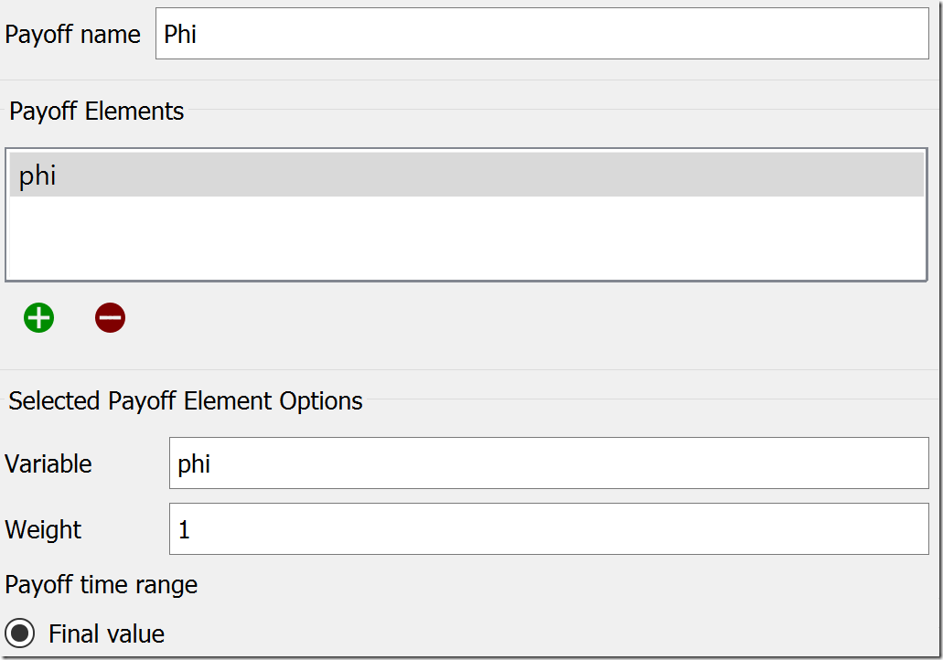
There are three tabs at the top of this tab:  Sensitivity, Payoff, and Optimization. We will use the latter two to configure the optimization. Starting on the Payoff tab, set the Payoff Name to “Phi” and add the variable phi to the list of Payoff Elements by clicking the green plus under that list. The other settings will remain at their default values, so it appears like this:

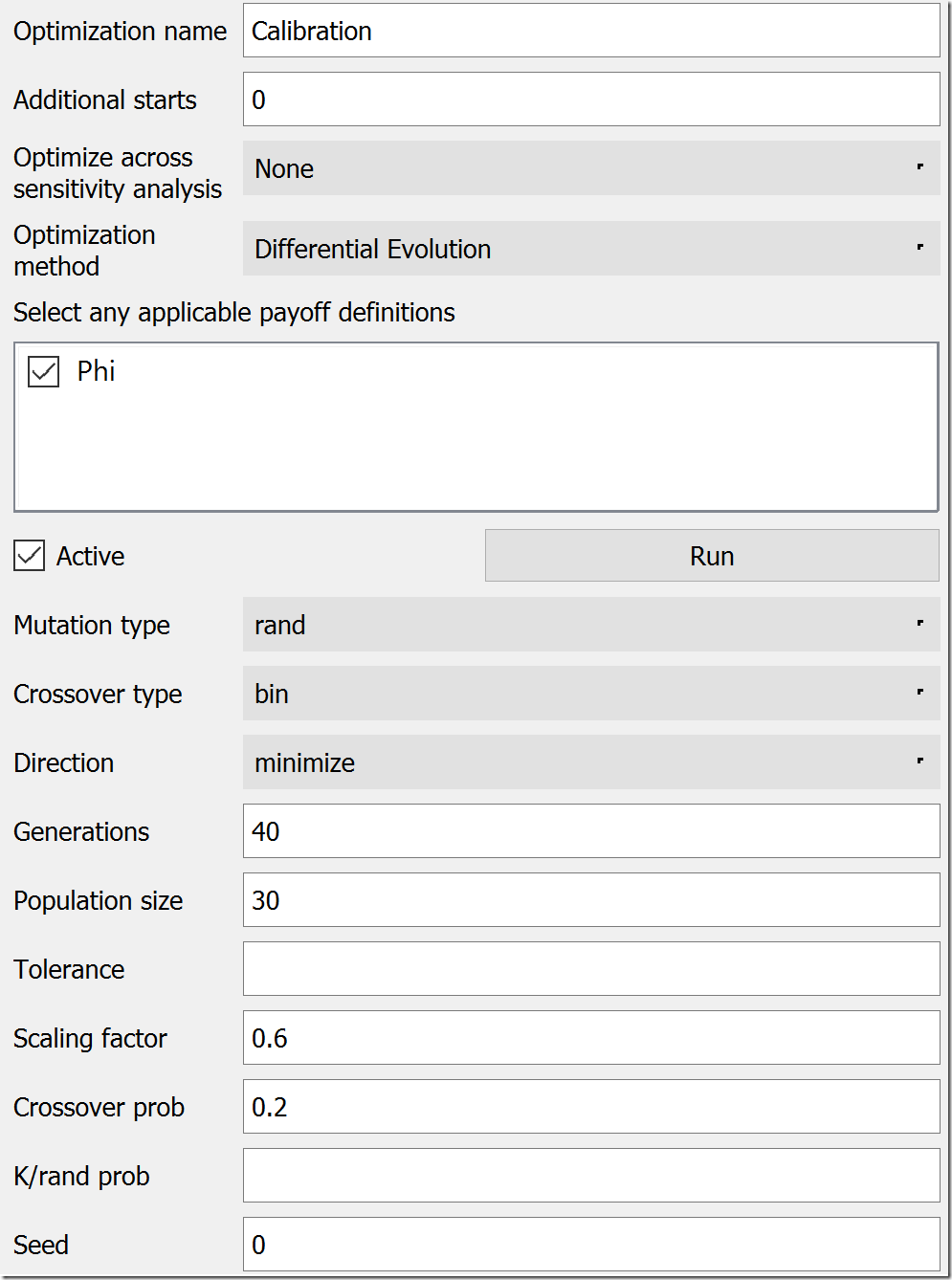
Next, we move to the Optimization tab. We could leave the default name of “Optimization,” but, to be clear, let’s rename it “Calibration.” Under Optimization Method, choose “Differential Evolution.” In the list below the method, check “Phi” as your payoff definition. DE has a lot of parameters, but the most of the defaults are a good starting place. Under Direction, change “maximize” to “minimize,” bump Generations to 40, and increase Population size to 30. Lower values will work, but these will give us consistent results for this model. At this point, the settings should look like this:

Scrolling down, we need to set up the parameters that will be varied. If you remember, these will be infection rate and recovery rate. In the last section of the panel, under Optimization Parameters, click the green plus button to first add infection rate. While it is selected, set its Min Value to 0 and its Max Value to 10 (below the list). Repeat this procedure for recovery rate, setting its Min Value to 0.1 (a 10-week recovery period) and it’s Max Value to 1 (a one-week recovery period). Make sure both of these parameters are now in the Optimization Parameters list.

Click in any area of the diagram to deselect the panel. You should notice an O-Run button in the lower left corner of the diagram, just to the left of the play button. Click it to start the optimization. you should see the graph below, which matches the PEST result. The Simulation Log Panel should also have opened (if not, choose it from the Window menu). You will see that the final value of phi is 4785.7, identical to what we got with PEST.

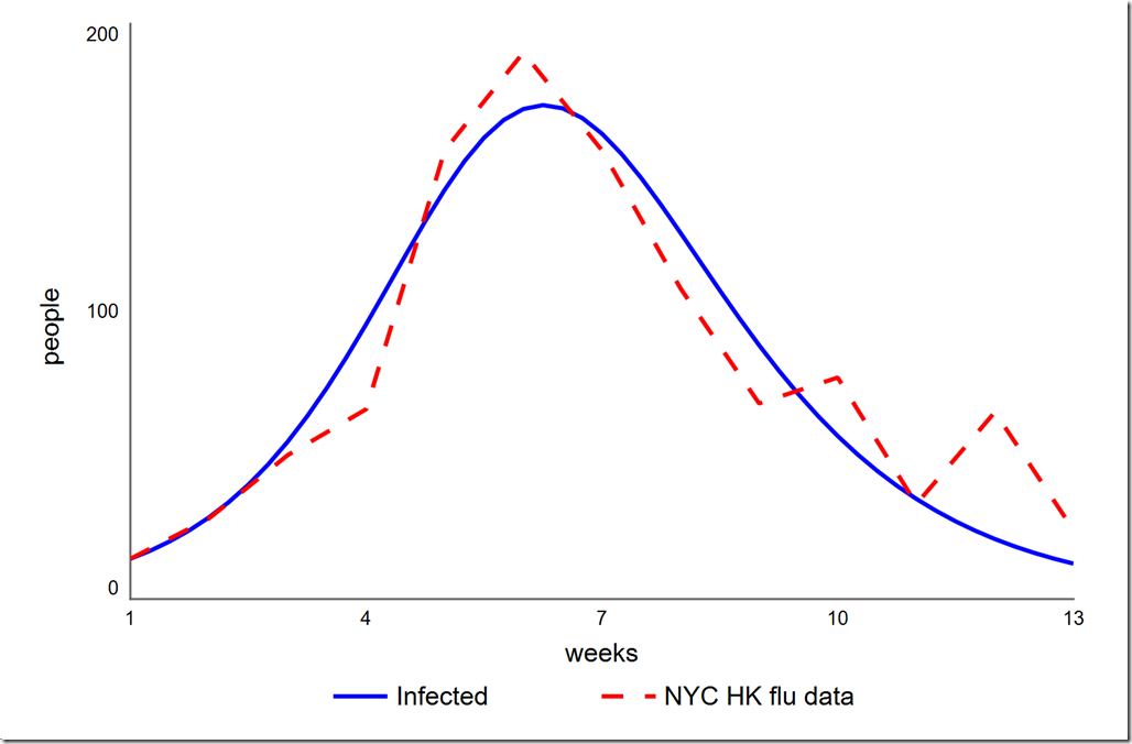
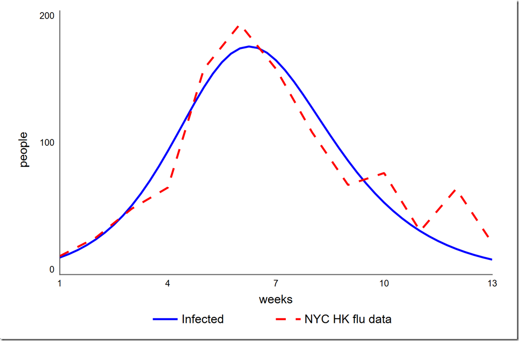
Earlier I said that we didn’t need to treat the initial value of Infected as a parameter since we knew its value. However, could we get a better overall calibration (which we have defined as a lower SSE) if we let it float? To test this, we have to add a variable initial infected to the model and set it to the value in the Infected stock (14). We then have to change the equation of Infected to initial infected (this is necessary because you cannot directly optimize a stock’s initial value). Once we’ve set this up, we can add initial infected to the Optimization Parameters on our Calibration setup on the Optimization panel. I used a range of 1 to 20, which yielded a slightly lower phi of 4765.6. The graph is shown below. Note the initial value of Infected is now 12.9 instead of the 14 given in the data. I don’t think that small improvement (0.4%) in our chosen metric is worth moving the one data point we always hit.

Considerations when using DE

Using this simple model, let’s explore some aspects of DE. DE is largely controlled by the scaling factor, F, which typically ranges from 0 to 1. Smaller values of F lead to greater exploration of the fitness landscape while larger ones lead to exploitation of solutions already found (i.e, quicker convergence). There is a very real tradeoff between computation time required and probability of success (converging to the global optimum). For some fitness landscapes, setting F too high will lead to premature convergence at a local minimum.

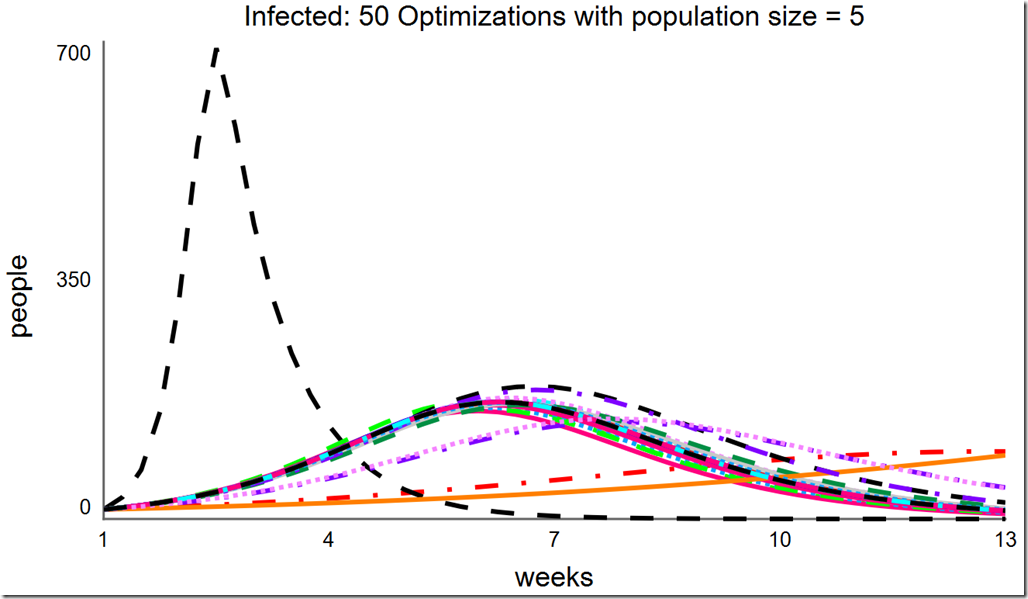
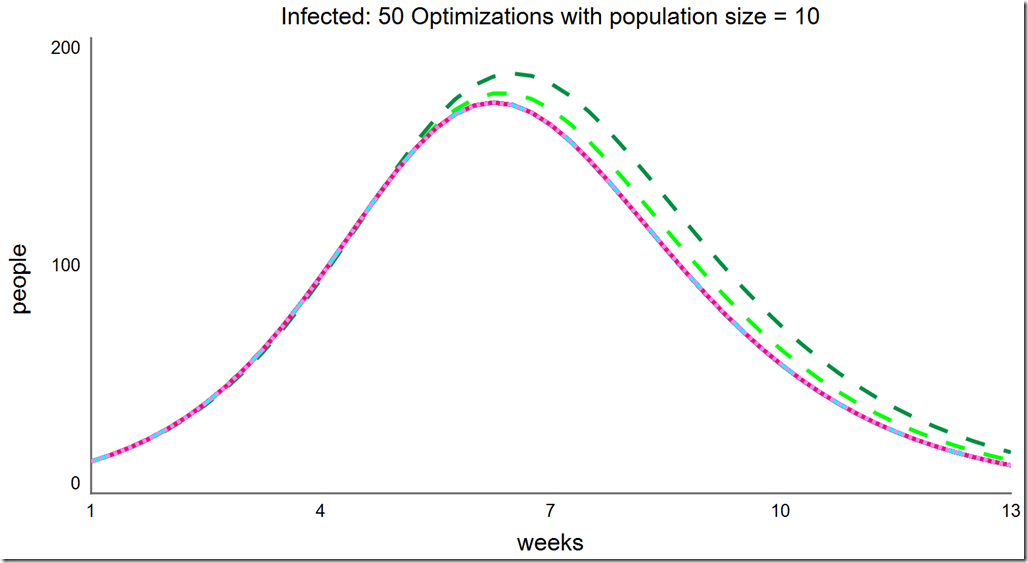
Another parameter that trades off these two factors is the population size. If the population is too small, there will not be enough diversity and DE will prematurely converge to a local minimum. If the population is too large, you will unnecessarily waste computation time. I have solved difficult two-objective optimizations with populations sizes as low as 60. Some single-objective problems can be solved with populations of 10 or fewer.

Finally, the number of generations affects whether the optimization runs long enough to converge. This should be long enough to get a decent solution, but not so long as to waste time. An alternative approach is to set this parameter high and also define the relative tolerance, which detects convergence.

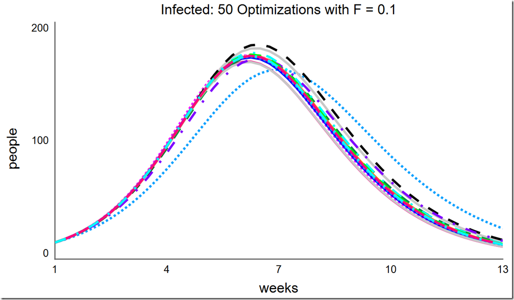
Let’s explore the effects of changing F and changing the population size. Recall the default value for F is 0.6.  If F is reduced to 0.1, the optimization converges at different minima:

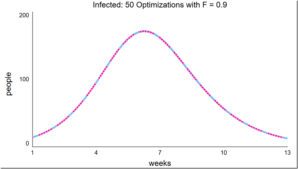
However, increasing F to 0.2 and above once again leads to consistent convergence at the global optimum:

Lowering the population size to 5 can save a lot of computing resource, but notice how many different local minima are captured with the reduced population diversity:

Increasing the population size to 10 improves the situation.  Here, it finds the global optimum almost all of the time, but as there are still some failures, we cannot be certain we’ve found the global optimum without running it multiple times:

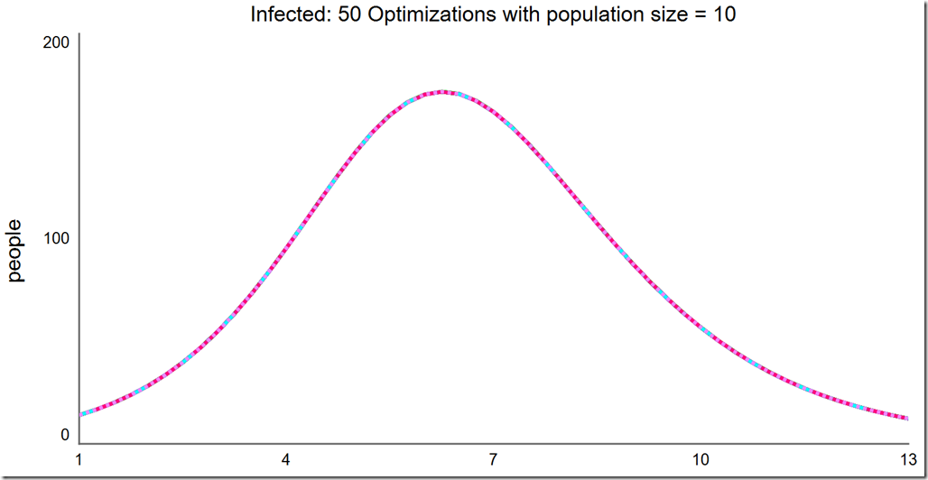
Note that the frequency of success is quite high at this small population size. Running another 50 optimizations, we see every one succeeded:

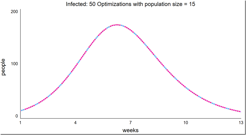
Finally, a  population of 15 always converges to the global optimum:

What about Powell?

As one final test, let’s compare these results to Powell. To do this we must first change the Payoff to have a weight of –1 instead of 1 (this causes Powell to minimize – we could do the same for DE, but it makes all of the objective values negative):

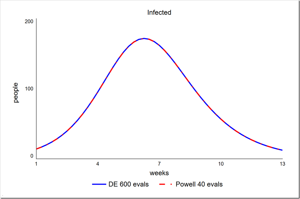
Powell get a phi of 4785.7 in just 40 runs, compared to 4785.7 in 600 runs using DE (30 generations with a population size of 20). Note that the parameters chosen for DE in this test (smaller than those used above) do not uniformly lead to an SSE of 4785.7 – sometimes it’s 4785.8 or 4785.9. More runs would lead to more uniform results. Note also that a lower population size of 15 (450 runs instead of 600) yields only slightly more variation. In contrast, Powell always gets 4785.7.

Why does Powell find the answer with far fewer runs? The answer has to do with the shape of the fitness landscape. Powell is a local hill climber and this function has a very sharp non-linear rise to a peak – an ideal problem for Powell. It is true that when DE is in exploitation mode it is also hill climbing, but it is looking at many different regions at once, trying to improve its chances of finding the global optimum.

Stay tuned next time to learn how to solve a single-objective optimization problem.