Modeling a Watershed with Arrays
This is the second installment of a four-part series. The other three parts can be accessed by clicking on the links below.
Methods for Using Arrays Effectively
Modeling Customers Switching Between Brands
Modeling Customers Switching Between Brands – The General Case
This is the second installment of a multipart series. The first part can be found by clicking here. Part 3 is available here.
In the first post of this series, I showed how to conditionally pull information from an array. In this post, I will extend this concept to show how to route information through an arrayed model. This is especially useful in spatial modeling applications.
Routing Water Through a Watershed
A common ecology application is the modeling of a watershed. Part of such a model will necessarily involve a network of stream or river segments – called reaches – which feed each other. It is desirable to implement this in a way that makes it easy to modify the reach network. Using an explicit stock-flow network makes this very difficult. However, it is relatively straightforward to use arrays of stocks and flows to build an easily configurable network.
Imagine a small watershed broken down into reaches as shown below:
![clip_image001[6] clip_image001[6]](https://blog.iseesystems.com/wp-content/uploads/2009/09/clip_image0016_thumb.gif)
For our purposes, a new reach will need to be created at every junction point. Therefore, in this example and from a topological point-of-view, it is not strictly necessary to treat reach 4 separately from reach 2 nor reach 5 separately from reach 3, but reaches 2 and 3 must be separate from reach 1. There are, of course, other reasons to separate reach 4 from 2 and reach 5 from 3, for example, slope, channel width, length, etc.
Every reach flows into exactly one other reach at its head, but many reaches can flow into the head of the same reach. This requires a many-to-one representation of the reach network. This is accomplished quite easily with a routing map which, for each reach, contains the number of the reach that this reach flows into. We also need someway to signify the outlet. Since reach numbers start at one, we can use zero to signify the outlet. Using these rules, the above network is completely represented in the following routing map:
| Reach | Flows into |
| 1 | 0 |
| 2 | 1 |
| 3 | 1 |
| 4 | 2 |
| 5 | 3 |
The nice thing about this representation is that it fits nicely into a one-dimensional array where the array index is the reach number and the reach it flows into is the value stored in that array element.
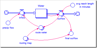
The model itself uses one stock to represent each reach. That stock has one inflow for water entering the reach and one outflow for water leaving the reach: (Download the zipped STELLA model here)

The Routing Magic
The outflow of one reach is directed to the next through the two-dimensional array route water. This array is arranged by placing outflows on the rows and inflows on the columns. Thus, outflowing amounts are placed one per row in the proper column for the reach it is headed for. This means there can only be one non-zero value in each row (but many per column). For example, at one point in the simulation, the array route water contains these values:
| From\To | 1 | 2 | 3 | 4 | 5 |
| 1 | 0.00 | 0.00 | 0.00 | 0.00 | 0.00 |
| 2 | 1.04 | 0.00 | 0.00 | 0.00 | 0.00 |
| 3 | 0.87 | 0.00 | 0.00 | 0.00 | 0.00 |
| 4 | 0.00 | 0.33 | 0.00 | 0.00 | 0.00 |
| 5 | 0.00 | 0.00 | 0.24 | 0.00 | 0.00 |
As expected, there is at most one non-zero value for each row. There is no non-zero value in the first row because that corresponds to the outlet, so no water is routed to another reach. The value in the second row is the outflow from reach 2, the value in the third is the outflow from reach 3, and so on. The columns sum to the amount of water being fed to the given reach. So reach 1 will receive 1.04 + 0.87 = 1.91, reach 2 will receive 0.33, and reach 3 will receive 0.24. Reaches 4 and 5 receive no inflow because they are at the top of the watershed (there are no reaches feeding into them).
The equation that does this magic is:
IF (routing_map[Reaches] = ARRAYIDX(2))
THEN outflow[Reaches]
ELSE 0
This says that when the column number (ARRAYIDX(2)) equals the reach number of the downstream reach (routing_map[Reaches]), fill the cell with that reach’s outflow. Note that we at most define one downstream reach for each reach, so this will only be non-zero in only one column. In this way, we avoid violating conservation of water.
The inflow then needs to sum the columns to get the total flow directed into that reach:
ARRAYSUM(route_water[*,Reaches])
The outflow at the stream outlet is captured in the converter final outflow, which has the equation:
ARRAYVALUE(outflow[*], ARRAYMINIDX(routing_map[*]))
This picks up the outflow value of the reach that has the smallest entry in the routing map. Since we defined the outlet to have the smallest value, zero, as long as we do not accidentally give two entries a zero value in the routing map, ARRAYMINIDX will find the array index (i.e., reach number) of the outlet.
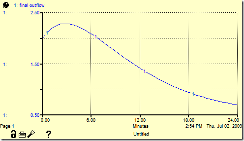
With constant precipitation, the behavior of the model at the end of a storm event appears below:

Extending the Model
This particular example has two simplifications that are easy to extend. The average time it takes water to flow through a reach (avg reach length in minutes) is constant, but can be made an array with different values for each reach. These values can also be calculated as the simulation progresses based on existing conditions in the reach. There is also a constant precipitation to all reaches all the time to keep water flowing into the system. This can be replaced by an array and a more intricate model of how precipitation flows into the stream over the landscape, or by a simple time series using a graphical function.
One final note about the model: I chose a stock with an average residence time to represent each reach. Under some circumstances, this may generate results that are confusing. For example, because it is an average residence time that follows an exponential distribution, some water that appears at the top of a reach will immediately exit from the bottom of the reach and other water that enters the reach will exit long after the average time has expired. In individual circumstances, for example a single short storm event, this representation may not match the real world very well. However, on average, over a long enough period of time, it matches the real behavior quite closely.
One alternative that enforces an exact delay for water moving across each reach is a conveyor. However, a conveyor is discrete in its behavior, so the model will not behave as true water flow does, i.e., continuously. Three stocks, i.e., a third-order material delay, could also be used for each reach to reduce the amount of entering water that exits immediately. Although this does cause the model to retain more water at the start of an event, it also leads to water being lost more quickly at the end.
Next time, I will use this same structure to model customers switching between different brands.