Modeling Customers Switching Between Brands – The General Case
This is the last installment of a four-part series. The first three parts can be accessed by clicking on the links below.
Methods for Using Arrays Effectively
Modeling a Watershed with Arrays
Modeling Customers Switching Between Brands
Generalizing the Model
When I showed Steve Peterson (at Lexidyne) my brand switching model, he told me there is a more general version that separates the customer loss fraction from the fraction won by another competitor. This has been presented in Pharmaceutical Product Strategy by Mark Paich, Corey Peck, and Jason Valant.
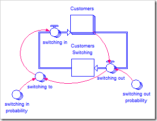
In my original formulation, the switching probability matrix was the product of these two variables. However, in many practical cases, the data available comes from two different places and reflects these two separate components. The revised model structure is shown below.

Instead of one composite switching probability, this model uses a switching out probability that is distinct from the switching in probability. The switching out probability is a one-dimensional array that, for each product, contains the fraction of customers lost to rivals every time unit (in our case, month). A sample for the five brands A, B, C, D, and E appears below.
| Brand | Fraction Lost |
| A | 0.091 |
| B | 0.170 |
| C | 0.046 |
| D | 0.026 |
| E | 0.071 |
switching out probability
We can see from this table that Brand B is losing 17% of its customers to rivals each and every month! Whoever is managing that product had better do something quickly.
The other side of the story has to do with which brand the customers are switching to. The switching in probability matrix contains, for each brand, the fraction of lost customers that migrate to a rival brand. Thus, each row of this matrix must add up to one (100% of lost customers). A sample appears below.
| From\To | A | B | C | D | E |
| A | 0.00 | 0.11 | 0.33 | 0.55 | 0.01 |
| B | 0.18 | 0.00 | 0.29 | 0.41 | 0.12 |
| C | 0.22 | 0.02 | 0.00 | 0.44 | 0.32 |
| D | 0.04 | 0.00 | 0.77 | 0.00 | 0.19 |
| E | 0.02 | 0.07 | 0.28 | 0.63 | 0.00 |
switching in probability
Note the diagonal will always be zero.
We can determine a lot of things from this table. For example, brand B offers no competition to brand D, brand D is the biggest rival of all the other brands, and brand C is brand D’s biggest rival.
Given these probabilities, we can find the number of customers switching out with the equation:
switching_out_probability[Products]*Customers[Products]
We can then use the exact same formulation as previously for switching to:
switching_out[Products]*switching_in_probability[Products, Products]
and switching in:
ARRAYSUM(switching_to[*, Products])
Note that all customers that switch between two brands also pass through a stock called Customers Switching. This was Steve Peterson’s idea: If the equations in the model are correct and all rows of switching in probability add up to one, as they ought to, this stock will always be zero. If it is ever non-zero, you immediately know there is something wrong with the numbers in switching in probability. [Note: Due to truncation errors during the simulation, the stock will not identically equal zero, so it has been globally scaled from –1 to +1 using the Range Specs.]
Expanding the Model
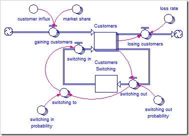
The structure given above models rivalry for existing customers quite well. However, it does not include flows for new customers entering the market or existing customers leaving the market. The full structure for acquiring and retaining customers looks like this (and is available by clicking here):

New customers are gained by each brand based on their respective market shares. Each brand also has a fraction of customers who are lost completely to this market, who perhaps move on to other technology or just stop using that type of product.
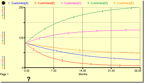
The simulation results are shown below for the case where all products start with 100 customers, no new customers are added, and the loss rate is zero.

Switching Based on Market Shares
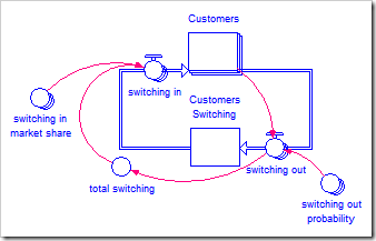
There is one further variant to customer brand switching that may be useful in some circumstances (it is available by clicking here):

In this version, rather than using a switching in probability, the number of customers gained each unit time is determined by a dynamic overall market share, the one-dimensional array switching in market share. Whereas the previous model (above) includes a mechanism whereby brand X explicitly gains customers from brand Y, this model bases switching on market share dynamics; if a customer decides to stop using brand X, they might then go searching for a replacement and would be more likely pick the market leader. Note the switching in market share can be the same as the brand’s overall market share or, as shown, it can reflect the different market shares between new customers (market share) and switching customers (switching in market share).